.md .pdf

repository open issue

Contents

Magnetohydrodynamics

Magnetohydrodynamics describes the dynamics of electrically conducting fluids in the presence of a magnetic field $\vec B$. The basic process that we are examining is:

• The $\vec B$ field idnuces currents in a moving, conducting fluid. The current in turn creates forces on the fluid, and also changes the $\vec B$ field. We add some aditional terms to the Navier-Stokes equation, and we couple those terms with Maxwell’s Equations.

Maxwell’s Equations

Maxwell Equations

$$\vec \nabla \cdot \vec E = 4\pi \rho_e \text{ Coulomb's Law}$$

• $\rho_e$ is charge density.

$$\vec \nabla \cdot \vec B = 0$$

$$\vec \nabla \times \vec E = \frac{1}{c}\frac{\partial \vec B}{\parital t} \text{ Faraday's Law of Induction}$$

• a time-varying $\vec B$ induces an electric field.

$$\vec \nabla \times \vec B = \frac{4\pi}{c}\vec{J} + \underbrace{\frac{1}{c}\frac{\partial \vec E}{\partial t}}_\text{displacement current} \text{ Ampere's Law }$$

• $\vec{J}$ is the current density

Some Comments

• Units:

  • Gaussian

    • This is what we use.

    • $E$ and $B$ are in the same units here.

  • SI

    • $[E] \sim [v\cdot B]$

• Charge and Current Densities

  • $\rho_e \sim \frac{\text{charge}}{\text{volume}}$

  • $\vec J \sim \frac{\text{charge}}{\text{volume}} \vec v = \rho_e \vec u$ where $\vec u$ is the electron velocity.

• Combining Maxwell’s Equations:

  • Let’s combine Coulomb’s Law + Ampere’s law by taking the divergence of Ampere’s Law:

$$\vec \nabla \cdot (\vec \nabla \times \vec B) = 0 = \frac{4\pi}{c} \vec \nabla \cdot \vec J + \frac{1}{c}\frac{\partial}{\partial t} \left(\underbrace{\vec \nabla \cdot \vec E}_{4\pi \rho_e}\right)$$

And thus we get charge conservation! ($\vec J = \rho_e \vec u$)

$$\boxed{\frac{\partial \rho_e}{\partial t} + \vec \nabla \cdot \vec J = 0}$$

• For steady-state current ($\partial_t \rho_e =0$, $\partial_t \vec E = 0$), then $\vec \nabla \cdot \vec J =0$.

  • We also have that Ampere’s Law becomes:

$$\vec \nabla \times \vec B = \frac{4\pi}{c}\vec J$$

Taking the divergence:

$$\vec \nabla \cdot \vec J = 0$$

which is consistent with what we had before. Here’s the important part: Maxwell realized that, without the displacement current term, we would only be allowed to have steady-state field (time variation not allowed).

• In the absence of sources for $\vec J$, Ampere’s law becomes:

$$\vec \nabla \times \vec B = \frac{1}{c}\frac{\partial \vec E}{\partial t}$$

Let’s take the curl:

$$\vec \nabla \times \left( \vec \nabla \times \vec B\right) = \frac{1}{c}\frac{\partial }{\partial t}\left(\vec \nabla \times \vec E\right) = -\frac{1}{c^2}\frac{\partial^2 \vec B}{\partial t^2}$$

Using vector identities:

$$-\nabla^2 \vec B + \vec \nabla(\underbrace{\vec\nabla\cdot\vec B}_{=0}) = -\frac{1}{c^2}\frac{\partial^2 \vec B}{\partial t^2}$$

And thus:

$$\boxed{\left(\nabla^2 - \frac{1}{c^2}\frac{\partial^2}{\partial t^2}\right)\vec B = 0}$$

We get a wave equation! And we get the same for a $\vec E$ field as well.

Ohm’s Law and Induction Equation for the Magnetic Field

Ohm’s Law is an empirical law, describing the relation between electric current and electric field (the Engineer’s Version):

$$I = \frac{V}{R}$$

This often fails at high $\vec E$.

1. In the rest frame of the conducting material: $\vec J^\prime = \sigma \vec E^{\prime}$, where $\prime$ denotes we are in the rest frame. Here, $\sigma$ is the electric conductivity, with units of $\frac{1}{\text{time}}$. We have:

$$J \sim \frac{1}{A}, E\sim \frac{V}{L} \rightarrow \text{ Ohm's Law: } \frac{I}{A} \sim \sigma \frac{V}{L} \rightarrow V \sim \frac{L}{A\sigma}I \equiv RI$$

Thus:

$$\sigma = \frac{L}{A\sigma} \rightarrow R \sim \frac{L}{A\sigma} \sigma \frac{1}{L\sigma} \propto \frac{1}{\sigma}$$

Resistance is inversely propotional to conductivity.

2. In the lab frame (an intertial frame), the conductor is moving at $\vec v$. We will show that, in this case,

$$\vec J = \sigma \left(\vec E + \vec v\times \frac{\vec B}{c}\right)$$

For a perfect conductor, meaning that $\sigma \rightarrow \infty$, we have:

$$\vec E + \vec v \times \frac{\vec B}{c} = 0 \rightarrow \vec E \perp \vec B$$

We also have:

$$|\vec E | \sim \frac{v}{c}|\vec B| \ll |\vec B|$$

We now have three equations (Ohm’s Law, Faraday’s Law, Ampere’s Law) and three unknown vector fields ($\vec B, \vec E, \vec J$). We combine these equations to get a single equation for $\vec B$, giving the induction equation.

Start with Ohm’s Law:

$$\vec E = \frac{\vec J}{\sigma} - \frac{\vec v \times \vec B}{c} \underbrace{\rightarrow}_\text{Ampere + ignore displacement current} \frac{c}{4\pi \sigma}\vec \nabla \times \vec B - \frac{\vec v \times \vec B}{c}$$

We now use Faraday’s Law:

$$\frac{\partial \vec B}{\partial t} + c \vec \nabla \times \vec E = 0$$

We now have:

$$\frac{\partial \vec B}{\partial t} + \frac{c^2}{4\pi \sigma}\vec v \times \left(\vec \nabla \times \vec B\right) - \vec \nabla \times (\vec v \times \vec B) = 0 \text{ assuming that } \sigma \text{ is spatially constant}$$

Last time, we looked at $\vec \nabla \times (\vec \nabla \times \vec B) = -\nabla^2 \vec B + \vec \nabla (\underbrace{\vec \nabla \cdot \vec B}_{0})$

And thus gives:

The Induction Equation – the evolution equation for B fields

$$\boxed{\frac{\partial \vec B}{\partial t} = \vec \nabla \times \left(\vec v \times \vec B\right) + \eta \nabla^2 \vec B}$$

where

$$\eta \equiv \frac{c^2}{4\pi \sigma}$$

is the “magnetic diffusivity” which is proportional to resistance.

This equation above is similar to the NS equation, by the way! And it motivates the introduction of the magnetic Reynold’s number. First, recall the hydrodynamical Reynold’s number:

$$\mathcal{Re} = \frac{vL}{\nu}$$

Similarly,we can define:

$$\mathcal{Re}_{m} \sim \frac{|\vec \nabla \times (\vec v\times \vec B)|}{|\eta \nabla^2 \vec B|}$$

Dimensionally, we have:

$$\mathcal{Re}_{m} \sim\frac{vB/L}{\eta B/L^2} \sim \frac{vL}{\eta}$$

where $v$ is the velocity, $L$ is the lenght of a typical variation of $\vec B$, and $\eta$ is the magnetic diffusivity/magnetic resistance.

We thus have two regimes, the low and high (magnetic) Reynold’s number regions:

1. Low $\mathcal{Re}_{m}$ has diffusion dominating:

$$\frac{\partial \vec B}{\partial t} \approx \eta \nabla^2 \vec B$$

And we can estimate the timescale for field decay due to diffusion:

$$\frac{B}{\tau} \sim \frac{\eta B}{L^2} \rightarrow \tau \sim \frac{L^2}{\eta}$$

2. Convective term dominates: this happens when we have really large conductivity (no resistance). This is the ideal MHD limit. Many astrophysical systems are well-described in this regime.

$$\frac{\partial \vec B}{\partial t} \approx \vec \nabla \times (\vec v\times \vec B)$$

---

We continue here from last time. We had the magnetic Reynold’s Number:

$$\mathcal{Re}_{m} \sim \frac{vL}{\eta}$$

where $\eta$ is our magnetic diffusivity vs. our classic Re:

$$\mathcal{Re}\sim\frac{vL}{\nu}$$

Examples of Conducting Fluids

• Astrophysical systems typically have $\mathcal{Re}_{m} \gg 1$.

• This is the “ideal MHD” limit.

	L [m]	v [m/s]	$\eta$ [m$^2$/s]	$\tau \sim L^2 / \eta$ (field decay time)	$\mathcal{Re}_{m}$
Mercury	0.1	0.1	1	0.01	0.01
Liquid Sodium	0.1	0.1	0.1	0.1	0.1
Earth’s Core	$10^{7}$	0.1	1	$10^{14} \sim 3$ million years	$10^6$
Sun’s Corona	$10^7$	$10^{3}$	1	$10^{14} \sim 3$ million years	$10^{10}$
ISM	$10^{17}$ (3 pc)	$10^{3}$	$10^{3}$	$10^{31}$	$10^{17}$

What does this mean? For high magnetic Reynold’s number, we have:

$$\frac{\partial \vec B}{\partial t} \approx \vec \nabla \times (\vec v \times \vec B)$$

And remember the vorticity from the Bernoulli law:

$$\vec \omega = \vec \nabla\times\vec v$$

We had re-written the Euler equation, and had:

$$\frac{\partial \vec \omega}{\partial t} = \vec \nabla \times (\vec v \times \vec \omega)$$

This is the Kelvin vorticity theorem.

This statement is a restatement of angular momentum, which has the same form as the magnetic equation we had above. What does this equation mean though?

• We have the flux of $\vec B$ or $\vec \omega$, equivalently, is conserved, and it moves along with the fluid. We can thus think of the magnetic field as being in “frozen in” with the fluid.

Lorentz Force

• The force on a charged particle moving with velocity $\vec u$ in a charged $\vec E$ and $\vec B$ field is given by:

$$\vec F = q\vec E + q \frac{\vec u}{c}\times \vec B$$

• Note: we now move to force density instead of force, dividing by volume.

$$\vec F = \rho_e \vec E + \frac{1}{c}\vec J\times \vec B$$

where $\vec J = \rho_e \vec u$. Typically in astrophysical systems, $\rho_e$ is very small (the material is almost always neutral), so we will ignore that term.

• We will also ignore the displacement current, allowing us to re-write $\vec J$ from Ampere’s Law:

$$\vec J = \frac{c}{4\pi} \vec \nabla \times \vec B$$

Note that, dimensionally, we have $B \sim \frac{v}{c}E \ll E$ for $v/c \ll 1$ (allowing us to drop the displacement current term).

Making these assumptions, we return to the force density equation:

$$\vec F = \frac{1}{4\pi}(\vec \nabla \times \vec B)\times \vec B = \frac{1}{4\pi} \left(-\frac{1}{2}\vec\nabla B^2 + (\vec B \cdot \vec \nabla)\vec B\right)$$

And we can now add this to the RHS of the Navier-Stokes equation:

Ideal MHD Navier-Stokes Equation

$$\boxed{\frac{\partial \vec v}{\partial t} + \left(\vec v \cdot \vec \nabla\right)\vec v = -\frac{1}{\rho}\vec \nabla\left(P + \frac{B^2}{8\pi}\right) - \vec \nabla \Phi + \frac{1}{4\pi \rho} \left(\vec B \cdot \vec \nabla\right) \vec B + \nu \left(\nabla^2 \vec v + \frac13 \vec \nabla(\vec \nabla \cdot \vec v)\right)}$$

• Let’s make sense of the new terms. Note that the $B^2 / 8\pi$ term represents magnetic pressure, since this is the energy density of the $B$-field. Magnetic fields do not like to be squeezed together, in the same way molecules don’t want to be squeezed! Thus, this is where the pressure comes from.

• The other new term $(\frac{1}{4\pi \rho} (\vec B\cdot \vec \nabla)\vec B)$ is called “magnetic tension.”

• We also hear about the “plasma $\beta$”-parameter, a measure of magnetic field strength relative to the pressure:

$$\beta \equiv \frac{P}{B^2/8\pi}$$

• In the weak-field limit, we have $\beta \gg 1$ (such as the interior of the Sun).

• In the strong-field limit, we have $\beta \ll 1$ (such as the solar corona).

• $\beta \sim 1 \rightarrow$, such as the ISM.

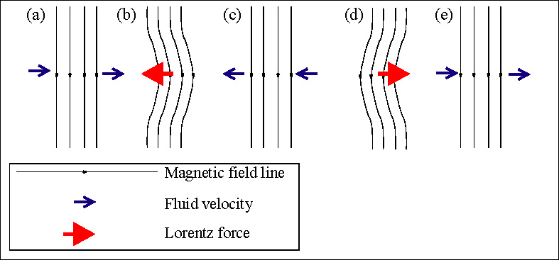
Two Types of $\vec B$ Forces

• (1) Pressure Gradient Term: the magnetic pressure force points in the direction of decreasing magnetic field density ($\propto -\vec \nabla \frac{B^2}{4\pi}$). That is to say that a high $\vec B$ region pushes out against a lower $\vec B$ region. This wants to spread out the fields uniformly.

• (2) Magnetic Tension Term: $\frac{1}{4\pi \rho} (\vec B \cdot \vec \nabla) \vec B$:

  • For a straight-line magnetic field (not curved): $\vec B = B \hat{z}$. Note that because the divergence has to be $0$, the strength of $B$ cannot depend on $z$.

  • Now let’s bend the field! Let’s have $\vec B(x,z) = B_0 \hat{z} + B_1 (x,z) \hat{x}$. Let’s examine the weird $\vec B \cdot \vec \nabla$ piece:

    • We have: $(\vec B \cdot \vec \nabla) \vec B = (\vec B \cdot \vec \nabla) B_1 \hat{x}$. This term that we are left with is in the $\hat{x}$ direction! If we bend the magnetic field, this force is trying to straighten it back out!

---

We continue here from last time. We had the induction equation:

$$\frac{\partial \vec B}{\partial t} = \vec \nabla \times (\vec v \times \vec B) + \eta \nabla^2 \vec B$$

We also had the Lorentz force:

$$\vec F = \frac{1}{4\pi} ( \vec \nabla \times \vec B ) \times \vec B$$

Using vector identities:

$$\vec F = \frac{1}{4\pi}\left(-\frac12 \vec \nabla \vec B^2 + (\vec B \cdot \vec \nabla)\vec B\right)$$

And thus we had the NS equation:

$$\boxed{\frac{\partial \vec v}{\partial t} + \left(\vec v \cdot \vec \nabla\right)\vec v = -\frac{1}{\rho}\vec \nabla\left(P + \frac{B^2}{8\pi}\right) - \vec \nabla \Phi + \frac{1}{4\pi \rho} \left(\vec B \cdot \vec \nabla\right) \vec B + \nu \left(\nabla^2 \vec v + \frac13 \vec \nabla(\vec \nabla \cdot \vec v)\right)}$$

We will take today to examine MHD waves!

Magnetohydrodynamical Waves

Let’s start by turning off a few things. Consider a non-viscous (inviscid), perfectly conducting fluid $(\sigma \rightarrow \infty)$ in a $\vec B$ field without gravity.

We now perform linear perturbations on densities, velocities, and the magnetic field:

$$\rho(\vec x, t) = \rho_0 + \rho_1(\vec x, t)$$

$$v(\vec x, t) = v_1(\vec x, t)$$

$$\vec B (\vec x, t) = \vec B_0 + \vec B_1 (\vec x, t)$$

Our continuity equation becomes:

$$\boxed{\frac{\partial \rho_1}{\partial t} + \rho_0 \vec \nabla \cdot \vec v_1 = 0}$$

And our NS equations becomes (using equation for F instead of vector identities):

$$\frac{\partial \vec v}{\partial t} + (\vec v \cdot \vec \nabla) \vec v = -\frac{1}{\rho}\vec \nabla P + \frac{1}{4\pi \rho}\left(\vec \nabla \times\vec B\right)\vec B$$

This is our original equation, let’s perturb it:

$$\boxed{\frac{\partial \vec v_1}{\partial t} = \frac{v_s^2}{\rho_0}\vec \nabla P_1 + \frac{1}{4\pi \rho_0} (\vec \nabla \times \vec B_1)\times \vec B_0}$$

We can now perturb our conduction equation:

$$\boxed{\frac{\partial \vec B_1}{\partial t} = \vec \nabla \times (\vec v_1 \times \vec B_0)}$$

We can combine the three boxed equations above:

We start by taking the time derivative of the perturbed NS equation:

$$\frac{\partial^2 \vec v_1}{\partial t^2} = v_s^2 \underbrace{\vec \nabla \left(\vec \nabla \cdot \vec v_1\right)}_\text{used first boxed eq} + \frac{1}{4\pi \rho_0}\left(\vec \nabla \times \underbrace{[\vec \nabla \times (\vec v_1 \times \vec B_0)]}_\text{from third eq boxed}\right) \times \vec B_0$$

We will now define a new velocity. We will define the Alfven speed/velocity:

Alfven Velocity

$$\vec v_A \equiv \frac{1}{\sqrt{4\pi \rho_0}}\vec B_0$$

This makes our equation:

$$\boxed{\frac{\partial^2 \vec v_1}{\partial t^2} - v_s^2 \vec \nabla (\vec \nabla \cdot \vec v_1) + \vec v_a \times \left(\vec \nabla \times [\vec \nabla \times (\vec v_1 \times \vec v_A)]\right) = 0}$$

We have three velocities here and four curls! What the hell is this? Let’s go to Fourier space…where $\vec \nabla$ becomes $\vec k$!

$$\vec v_1 (\vec x, t) = \int \mathrm{d}^3 k \, \vec v_1 (\vec k) e^{i (\vec k \cdot \vec r - \omega t)}$$

In $k$ space, we can re-write our nasty equation from above. $\partial t$ will give $i\omega$ each time.

$$-\omega^2 \vec v_1 + (v_s^2 + v_A^2)(\vec k \cdot \vec v_1)\vec k + \vec v_A \cdot \vec k\left((\vec v_A \cdot \vec k)\vec v_1 - (\vec v_1 \cdot \vec k)\vec v_A - (\vec v_A \cdot \vec v_1)\vec k\right) = 0$$

The non-zero terms depend on where we are pointing relative to $\vec k$. We breakdown our vector components into:

Longitudinal Magnetosonic Waves

1. For $\vec k \perp \vec v_a$ (recall that $\vec v_A \parallel \vec B_0 \rightarrow \vec k \perp \vec B_0$). In other words, these are modes perpendicular to the direction of the field. This makes our equation above:

$$\omega^2 \vec v_1 = (v_s^2 + v_A^2)k^2 \left(\vec v_1 \cdot \hat{k}\right) \hat{k}$$

The fluid equation tells us that $\vec v_1 \parallel \hat{k}$ and $\boxed{\omega^2 = (v_s^2 + v_a^2)k^2}$ This is a dispersion relative like free-sound waves, but with the extra magnetic pressure term. This is called longitudinal (in direction of k) magneto-sonic waves with phase velocity $v_{\phi} = \sqrt{v_s^2 + v_A^2}$, depending on both the hydrostatic and magnetic pressures. This makes sense since the $\vec B$ lines are “frozen” to the fluid and get compressed with the fluid.

Now remember our conduction equation! As we compress the magnetic field lines (squeezing them closer together). Our $\vec B_1$ comes form our pertubed conduction equation, and we get:

$$\vec B_1 = \frac{k}{\omega} v_1 \vec B_0$$

These waves are parallel to $\vec B_0$ and thus only change the strength of the magnetic fields, not the direction.

Parallel

2. For $\vec k \parallel \vec v_A \parallel \vec B_0$ , we return to our large equation above, and we get two types of wave-motions. We will call them (2i) and (2ii).

2i. Longitudinal $\vec v_1 \parallel \vec k \parallel \vec v_A \parallel \vec B_0$ (everyone is in the same direction). We return to our monster equation. Because we are all in the same direction, we can drop all vector signs. This gives:

$$-\omega^2 v_1 + (v_s^2 + v_A^2) k^2 v_1 - v_A^2 k^2 v_a^2 = 0$$

And the magnetic field term cancels!

$$\boxed{\omega^2 = v_s^2 k^2}$$

These are normal sound waves! And what happens to the perturbed $\vec B_1$ piece? $\vec B_1 = \vec 0$ since $\vec v_1 \times \vec B_0 = 0$ (assuming $\vec B_1(t=0)=0$. Waves which travel along the magnetic field lines do not actually feel the magnetic field!

Transverse

2ii. In this case $\vec k$ is still parallel but $\vec v_1$ is perpendicular to $\vec k$. This is to say that $\vec B_1 \perp \vec v_A$, and also that $\vec v_1 \perp \vec B_0$. Returning to our major equation:

$$-\omega^2 \vec v_1 + (v_A k)^2 \vec v_1 = 0 \rightarrow \boxed{\omega^2 = v_A^2 k^2}$$

These are pure MHD waves, something we have never seen before, and are called Alfven waves. For completeness, what happens to $\vec B_1$? From the conductivity equation, we have: $\vec B_1 = - \frac{k}{\omega} B_0 \vec v_1$.

$$\dot{\rho} = 0 \rightarrow \text{No density perturbations (from equation 1 above)!}$$

These waves travel up and down the magnetic field lines, shaking them left and right. They make the fluids wiggle around!

---

We continue here from last time. Recall from last time that we had three types of MHD waves:

1. $\vec k \perp \vec B_0$ ($\vec v_A \parallel \vec B_0$). Here we had magnetosonic waves (combination of the two below):

$$\omega^2 = (v_s^2 + v_A^2)^2$$

In this case, we had $\vec B_1 \parallel \vec B_0$ and $\vec v_1 \parallel \hat{k}$ and we had the $\vec B$ field compressing in space.

2. $\vec k \parallel \vec B_0$. Unlike previosuly, we have two cases where $\vec v_1$ is parallel or perpendicular to $\vec k$.

2i. $\vec v_1 \parallel \vec k$ (everything is parallel here since these are also $\propto \hat{z}$. In this case, we get pure sound waves:

$$\omega^2 = v_s^2 k^2$$

and

$$\vec B_1 = 0$$

giving us normal sound waves. If you are moving in the direction of $\vec B$, you don’t feel the $\vec B$ and thus we have normal sound waves.

2ii. $\vec v_1 \perp \vec k$. In this case, we get pure MHD waves:

$$\omega^2 = v_A^2 k^2$$

and

$$\vec B_1 \propto \vec v_1$$

The result here is that the $\vec B$ fields wiggle / the fluid is perturbed along the magnetic fields perpendicular to $\vec B_0$. These are sometimes called Alfven waves.

Remember back in early April where we were discussing disks? Let’s return there.

Magneto-Rotational Instability

Consider a razor thin accretion disk in a $\vec B = B_0 \hat{z}$ field in cylindrical coordinates. We are rotating with $\vec \Omega = \Omega \hat{\phi}$. The relevant MHD equations are:

$$\frac{D\vec v}{Dt} = -\frac{1}{\rho}\vec\nabla\left(P + \frac{B^2}{8\pi} \right) - \vec \nabla \Phi + \frac{1}{4\pi \rho} \left(\vec B \cdot \vec \nabla\right) \vec B$$

And the induction equation:

$$\frac{\partial \vec B}{\partial t} = \vec \nabla \times (\vec v \times \vec B)$$

(where the induction equation is in the perfect conductor limit). We can re-write this as :

$$\frac{\partial \vec B}{\partial t} = (\vec B \cdot \vec \nabla) \vec v - (\vec v \cdot \vec \nabla) \vec B + \vec v(\vec \nabla \cdot \vec B) - \vec B (\vec \nabla \cdot \vec v)$$

Two terms are $0$. We have $\vec \nabla \cdot \vec B = 0$ from Maxwell, and because we are incompressible, we have $\vec \nabla \cdot \vec v = 0$. Linear perturbation theory continues from here.

We perturb about the equilibrium state of a Keplerian accretion disk surrounding a massive object. This disk has a uniform, vertical $\vec B$ field given by: $\vec B = B_0 \hat{z}$. We consider small perturbations:

$$\vec u_0 \equiv \vec v - R \vec \Omega = 0 \text{ in rotating frame }$$

And we introduce

$$\vec u_1 \equiv \text{ perturbed fluid velocity in the rotating frame}$$

We also have:

$$\vec B = B_0 \hat{z} + \vec B_1$$

where $\vec B_1$ is the perturbed magnetic field. We now assume a solution of the form:

$$\vec u_1 \propto e^{i(kz - \omega t)}$$

and

$$\vec B_1 \propto e^{i(kz-\omega t)}$$

That is to say we are considering perturbation modes with $\vec k = k \hat{z} \parallel \vec B_0$ in the disk plane. By construction here, we are limit ourselves to the case when we get pure MHD waves. We will skip many lines of math.…

At the end of the day, we have four unknowns: $u_{1R},u_{1\phi}$ and $B_{1R},B_{1\phi}$ with 4 equations (MHD + Induction). In the end, we get the dispersion relatio for MRI:

Magneto-Rotational Instability

$$\omega^4 - \omega^2 \left(\kappa^2 + 2\left(k v_A\right)^2\right) + (kv_a)^2\left[(k v_A)^2 + \frac{d(\Omega^2)}{d\ln R}\right] = 0$$

where $\kappa$ is the epicylcic frequency we have discussed before. Let’s analyze what this equation means!

Some comments on the dispersion relation above

1. Turn off rotation. Remember earlier that rotation stabilizes disks. Do we find the same here? When we turn off rotation, we have $\kappa \rightarrow \Omega \rightarrow 0$. This leaves:

$$\omega^4 - 2(kv_a)^2\omega^2 = 0 \rightarrow (\omega^2 - k^2 v_A^2)^2 = 0 \rightarrow \omega^2 = k^2 v_A^2$$

We recover pure MHD waves!

2. Back to full dispersion relation….the disk is MRI-unstable if $\omega^2 < 0$. We can show in PS7 that $\omega^2 < 0$ if:

Instability Criterion for MRI

$$k^2 v_A^2 < -\frac{d(\Omega^2)}{d\ln R}$$

For Keplerian orbits, $\Omega \equiv \frac{v_\phi}{R} \propto \frac{1}{R^{3/2}} \rightarrow k^2 v_A^2 < 3\Omega^2$ is the condition for a Keplerian disk. Large wavelength $\lambda$ modes are thus MRI unstable. So rotation is actaully introducing instability!

3. Unstable modes grow with $e^{|\omega| t}$ . In PS7, we will show that there is maximum $\omega_{max}$. What is the correpsonding $k$ for $\omega_{max}$?

$$\omega_{max} \text{ occurs at } k_{max}^2 v_A^2 = -\frac14 \left(1+\frac{\kappa^2}{4\Omega^2}\right)\frac{d(\Omega^2)}{d\ln R}$$

For a Keplerian disk, we have:

$$\boxed{|\omega_{max}| = \frac{1}{2}|\frac{d\Omega}{d\ln R}|}$$

So….how fast is this? For a Keplerian disk, we have:

$$|\omega_{max}| = \frac34 \Omega$$

The orbital period is $2\pi /\Omega$, so these timescales are actually comparable! The instability is on the orbital timescale! This is very fast, with the growth factor giving:

$$\text{Growth } \propto e^{|\omega_{max}|t}$$

In 1 orbital period, $e^{\omega_{max}t} \sim e^{\frac34 \Omega \cdot \frac{2\pi}{\Omega}} \sim e^{1.5\pi} \sim 110!!!!!$.

This is the whole idea behind MRI! Within a few orbital periods, the magnetic fields enhance our initial amplitudes by factors of 100’s! We don’t have the same timescale issues from viscosity alone.

What is the physical picture here? What’s going on? Why does rotation induce instability?

• Inner orbits race ahead of the outer orbits! Importantly, though, the angular momentum $L \propto VR \propto R^2 \Omega$ and so the angular momentum actually grows with $R!$.

• As interior masses move ahead of exterior masses, the magnetic tension between the two makes the system lose angular momentum. This induces the interior mass to drop in orbit, and the outer masses moves outward!

• This is typically how people exlain MRI. Rotation helps because it causes this angular momentum transfer.

---

previous

Kinetic Theory

next

Turbulence