.md .pdf

repository open issue

Contents

Viscous Flows

Viscous Stress Tensor and the Viscous Force

Viscosity is a measure of of fluid “friction” – the resistance a material has to being deformed by sheer stress. Shear stresses can be pointing in every direction, but has a spatial gradient.

Water is wet. What does this mean? It really means that it’s viscous at the molecular level! Without viscosity, you would come out of a swimming pool totally dry. Can we “derive” viscosity from first principles? Kinda of.…

Heuristic: Miscroscopic/Molecular Origin of Viscosity

Viscosity arises from diffusive momentum transfer due to particle scattering. Consider a shear flow $\vec v = v_y(x)\hat{y}$. Note in the diagram below, the axes are labelled wrong. Rotate by 90 degrees. Consider the forces on a volume element $A \cdot \Delta x$.

Consider sitting at $x$, which is one of the flow arrows in the diagram below. At location $x$, particles receive momentum transfer from those at $x - \frac{l}{2}$ and $x+\frac{l}{2}$ where $l$ is the mean free path, and adjacent fluid elements are spearated by $\Delta x \gg l$.

Now consider particles at $x+ \frac{l}{2}$, which have $\hat{y}$-momentum of: $mv_y\left(l+\frac{l}{2}\right)$.

Now consider particles at $x- \frac{l}{2}$, which have $\hat{y}$-momentum of: $mv_y\left(l-\frac{l}{2}\right)$.

1. Thus the net $\hat{y}$-momentum transfer per particle across the boundary $x$ is:

$$p_y(x) \approx m \frac{\partial v_y}{\partial x} \cdot l$$

2. We want to consider the flux, now. We need the number of particles per unit time passing through $x$. This is simpy:

$$n \cdot v_{th} \cdot A \text{ where } v_{th} \sim \sqrt{\frac{kT}{m}}$$

is the typical thermal speed of these particles.

Together, these two points give the net momentum transfer through $\hat{x}$:

$$\dot{p}_y(x) \approx m \frac{\partial v_y}{\partial x} l \cdot n v_{th} A$$

Remind yourself what the time derivative of momentum is – it’s a force! We can now consider the net force between adjacent fluid elements.

The viscous force is the net force on element $A \cdot \Delta x$ by surrounding fluids. Thus,

$$F_y = \dot{P}_y (x+\Delta x) - \dot{p}_y(x) \approx \frac{\partial \dot{p}}{\partial x} \Delta x$$

We can use our expression for $p_y(x)$ from above. This gives:

$$F_y \approx A \cdot \Delta x \frac{\partial}{\partial x} \left(m \cdot n \cdot l \cdot v_{th} \cdot \frac{\partial v_y}{\partial x}\right)$$

And now the viscous force per unit volume can be written as:

$$\frac{F_y}{A \cdot \Delta x} \approx \frac{\partial}{\partial x} \left(\rho \cdot \nu \frac{\partial v_y}{\partial x}\right)$$

where $\rho = mn$ is the mass density, and $\nu = l v_{th}$ is the kinematic viscosity and has units of $\text{cm}^{2} \text{ s}^{-1}$. Sometimes, we combine terms even more:

$$\eta \equiv \rho \nu \equiv m\cdot n \cdot l \cdot v_{th}$$

where $\eta$ is called the dynamic viscosity. In this re-arrangment, we can write:

$$\frac{F_y}{A \cdot \Delta x} \approx \frac{\partial }{\partial x}\left(\eta \frac{\partial v_y}{\partial x}\right)$$

And lastly, we can group together the parentheses, giving:

$$\boxed{\frac{F_y}{A \cdot \Delta x} \approx \frac{\partial }{\partial x}\left(\sigma_{yx}\right)}$$

where

$$\boxed{\sigma_{yx} \equiv \eta \frac{\partial v_y}{\partial x} }$$

is called the viscous/shear stress “tensor.”

This derivation is almost correct, but not quite the whole story.

Constructing the Viscous Stress Tensor

Let’s try to contrusct the tensor from the start, with the condition that it is linear in the velocity gradient. This means:

$$\frac{\partial v_i}{\partial x_j} = \partial_j v_i \text{ for } i =1,2,3$$

The most general form is thus:

$$\sigma_{ij} \equiv \eta \left(\partial_j v_i + \alpha \partial_i v_j + \beta \delta_{ij} \underbrace{\partial_k v^k}_\text{divergence term}\right)$$

We can now apply some conditions to constraing $\alpha$ and $\beta$.

1. We know that $\sigma_{ij} = 0$ for a uniform, solid-body under rotation, i.e., no shearing/viscous force. For uniform rotation, we have:

$$\vec v = \Omega R \hat{\phi}$$

where $\phi$ is the polar-coordinate direction in the $x,y$ plane. Recall as well that: $\hat{r} = \cos \phi \hat{x} + \sin \phi \hat{y}$ and $\hat{\phi} = -\sin \phi \hat{x} + \cos \phi \hat{y}$. Let’s use this:

$$\vec v = \Omega R \left(-\sin \phi \hat{x} + \cos \phi \hat{y}\right) = -\Omega \left(y\hat{x} - x\hat{y}\right)$$

Let’s now look at the component $\sigma_{xy}$:

$$\sigma_{xy} \propto \partial_y v_x + \alpha \partial_x v_y \propto -1+\alpha = 0 \rightarrow \alpha = 1$$

2. Isotropically expanding fluid (Hubble Flow). In this case, we ALSO know that $\sigma_{ij} = 0$. The flow is radially outward, and thus we have no shear. In this case, we have $\vec v \propto \vec r \propto x \hat x + y \hat y + z \hat z$. We can immediately see that the ineresting case has $\sigma_{xx}$ or the like. All other terms vanish. We have:

$$\sigma_{xx} \propto 1 + \alpha + 3\beta = 0 (\text{ no shear })$$

And thus:

$$\beta = -\frac{1 + \alpha}{3} \rightarrow \beta = -\frac{2}{3}$$

3. We are finished! Let’s collect our results. We just showed that:

$$\sigma_{ij} = \eta \left(\partial_j v_i + \partial_i v_j - \frac{2}{3} \delta_{ij} \partial_k v^k\right)$$

Note that this is a traceless tensor of rank 2.

Navier-Stokes Equation and Reynold’s Number

Recall the stress tensor:

$$T_{ij} = \underbrace{P \delta_{ij} }_\text{ thermal pressure } + \underbrace{\rho v_i v_j}_\text{ram pressure} \underbrace{- \sigma_{ij}}_\text{viscous term}$$

Remember that momentum conservation (Euler’s Equation) tells us that:

$$\frac{\partial}{\partial t} (\rho v_i) = - \partial_j T_{ij} - \rho \partial_i \Phi$$

With our new viscosity term (per unit volume), we get a new piece to this equation:

$$\frac{\partial}{\partial t} (\rho v_i) = - \partial_j T_{ij} - \rho \partial_i \Phi + \partial_j \sigma_{ij}$$

And using our form for $\sigma_{ij}$:

$$\frac{\partial }{\partial t}\left(\rho v_i\right) = \eta \left(\nabla^2 v_i + \partial_i \left(\vec \nabla \cdot \vec v\right) - \frac23 \partial_{i} (\vec \nabla \cdot \vec v )\right) = \eta \left(\nabla^2 v_i + \frac13 \partial_i \left(\vec\nabla\cdot \vec v\right)\right)$$

Our momentum equation in our original form thus becomes the Navier-Stokes Equation:

Navier Stokes Equation

$$\frac{\partial \vec v}{\partial t} + (\vec v \cdot \vec \nabla) \vec v = -\frac{1}{\rho}\vec \nabla P - \vec \nabla \Phi \underbrace{+ \underbrace{\nu}_\text{kinematic viscos.}\left(\nabla^2 \vec v + \frac13 \vec \nabla (\vec \nabla \cdot \vec v)\right)}_\text{viscous force per unit mass}$$

Some comments….

1. For incompressible fluids, $\vec \nabla (\vec \nabla \cdot \vec v) = 0$.

2. Viscosity shows up in the momentum equation as a diffusion term, e.g.:

$$\frac{\partial \vec v}{\partial t} = \nu \nabla^2 \vec v$$

This should remind us of the drunkard’s walk, which makes sense since this comes from molecular momentum transfer. The typical form of the solution for 1D diffusion is:

$$\vec v(x,t) \propto \frac{1}{\sqrt{\nu t}}e^{-\frac{x^2}{4\nu t}}$$

3. You can add a traceful term into $\sigma_{ij}$ which manifests as a bulk-viscosity. We do this by:

$$\sigma_{ij} \rightarrow \sigma_{ij} + \gamma \delta_{ij} \partial_k v^k$$

for some phenomenonological forces.

4. Kinematic Viscosity $\nu$ (diffusion coefficient with units of length squared over time) for some materials at room temperature:

• Water has $\nu = 0.01 \text{ cm}^2 \text{ s}^{-1}$

• Air has $\nu = 0.01 \text{ cm}^2 \text{ s}^{-1}$

• Oil has $\nu = 1\text{ cm}^2 \text{ s}^{-1}$

• Syrup has $\nu \sim 1000\text{ cm}^2 \text{ s}^{-1}$

The Navier-Stokes Equation and Reynold’s Number

Recall the Navier-Stokes equation:

$$\frac{\partial \vec v}{\partial t} + (\vec v \cdot \vec \nabla) \vec v = -\frac{1}{\rho} \vec \nabla P - \vec \nabla \Phi + \nu\left(\nabla^2 \vec v+ \frac13 \vec \nabla (\vec \nabla \cdot \vec v)\right)$$

This motivates the Reynold’s number. The Reynold’s number is a dimensionless quantity which tells us if viscosity is relevant.

Reynold’s Number

$$\boxed{\mathcal{R} \equiv \frac{vL}{\nu}}$$

where $v$ is the typical flow speed, $L$ is the typical length scale, and $\nu$ is the viscosity. What are some typical values?

Well, consider stirring a cup of tea: $v\sim 5 \text{cm } \text{s}^{-1}$, $L \sim 5 \text{cm } \text{s}^{-1}$, $\nu \sim 0.01 \text{ cm}^{2} \text{ s}^{-1}$. This gives a Reynold’s $\mathcal{R} \sim 2500$.

But what does this number mean physically? Well, $\mathcal{R}$ is measuring the ratio of “inertial forces” to “viscous forces.” The inertial force is $\sim (\vec v \cdot \vec \nabla) \vec v \sim \frac{v^2}{L}$. The viscous force is $\sim \nu \nabla^2 \vec v \sim \frac{\nu \cdot v}{L}$, and $\mathcal{R}$ is sort-of like the ratio of these two terms – the inertial force over the viscous force.

$$\mathcal{R} \sim \frac{|(\vec v \cdot \vec \nabla) \vec v|}{|\nu \nabla^2 \vec v|} \sim \frac{vL}{\nu}$$

• When $\mathcal{R} \ll 1$, we say that viscosity is important.

• When $\mathcal{R} \gg 1$, we say that the fluid is “inviscid,” meaning non-viscous.

At low $\mathcal{R}$, flows tend to be laminar. At high $\mathcal{R}$, flows tend to be turbulent.

Applications: Examples of Viscous Flows

Example 1: Poiseuille Flow

This describes laminar, non-turbulent, constant flow of an incompressible uniform viscous fluid through a tube of constant cross section. An example of this would be blood flow in veins.

We start with the Navier-Stokes equation.

$$\underbrace{\frac{\partial \vec v}{\partial t}}_{0 \text{ bc const. flow} } + (\vec v \cdot \vec \nabla) \vec v = -\frac{1}{\rho} \vec \nabla P - \underbrace{\vec \nabla \Phi}_\text{ignore for now} + \nu\left(\nabla^2 \vec v+ \frac13 \vec \nabla (\underbrace{\vec \nabla \cdot \vec v}_\text{0 bc incompressible})\right)$$

Thus, our equation to solve is:

$$(\vec v \cdot \vec \nabla) \vec v = -\frac{1}{\rho} \vec \nabla P + \nu \nabla^2 \vec v$$

Let’s take the flow to be along the z-direction $\hat{z}$. Let’s let the velocity depend on $x$ and $y$, though. Thus:

$$\vec v = v(x,y) \hat{z} \rightarrow \text{ constant flow along } \hat{z}$$

By constuction, we have:

$$\frac{\partial v}{\partial z} = 0$$

but

$$\frac{\partial v}{\partial x} \text{ and }\frac{\partial v}{\partial y} \text{ need not be } 0$$

The left-hand side of the N.S. equation becomes:

$$v \frac{\partial }{\partial z}v = 0$$

Thus, the right-hand side of the N.S. equation must be $0$:

$$\nabla^2 v = \frac{1}{\rho \nu} \frac{\partial }{\partial z}P$$

Remember that $\rho \nu$ is the same thing as the kinematic viscosity $\eta$. Thus:

$$\nabla^2 v = \frac{1}{\eta}\frac{\partial}{\partial z}P$$

This is the same as:

$$(\partial_x^2 + \partial_y^2) v = \frac{1}{\eta} \frac{\partial}{\partial z} P$$

Notice that the left-hand side has no $z$ dependence. Thus, $\partial_z P$ has to be a constant!

$$\partial_z P = \text{const.} \equiv -\underbrace{\frac{\Delta P }{\Delta L}}_{\text{ pressure difference over length }\Delta L}$$

The right-hand side has no $x$ or $y$ dependence since $v_x$ and $v_y$ are zero by construction. Thus:

$$\partial_x P = \partial_y P = 0$$

We now look at the cross-section of the tube, and want to solve for the velocity profile.

We thus have:

$$(\partial_x^2 + \partial_y^2)v = \frac{1}{R}\frac{d}{dR} \left(R\frac{dv}{dR}\right) = -\frac{1}{\eta}\frac{\Delta P}{\Delta L}$$

Thus:

$$R \frac{dv}{dR} = -\frac{1}{\eta} \frac{\Delta P}{\Delta L} \left(\frac{R^2}{2} + a\right)$$

Simplifying and integrating one more time:

$$v(R) = -\frac{1}{\eta} \frac{\Delta P}{\Delta L} \left(\frac{R^2}{4} + a\ln R + b\right)$$

We now impose boundary conditions – one at the center and one at the boundary of the tube.

1. At $v(R=0)$, we want $v$ to be finite. This implies that $a=0$ since $\ln R$ grows to infinity.

2. At $v(R=R)$, we want the fluid to have no velocity. The only way for this to work out is for:

$$\boxed{V(R) = \frac{\Delta P}{4\eta \Delta L}\left(R_0^2-R^2\right)}$$

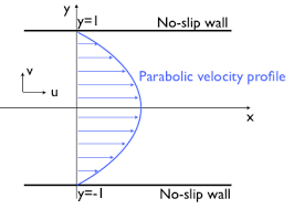
What does this mean, actually?

• We have a parabolic velocity profile!

• The maximum velocity is at the center of the tube.

• The maximum speed depends on the width of the tube. We have $V_{MAX} \propto R_0^2$. The wider the tube, the faster the flow.

Lastly, we can calculate the mass flux through the tube. To do this, we calculate:

$$\text{Mass flux through tube} = \int v\rho \, \mathrm{d}A$$

We have:

$$\text{mass flux } = 2\pi \rho \int_0^{R_0} v R \,\mathrm{d}R = 2\pi \rho \int_0^{R_0} \frac{\Delta P}{4\eta \Delta L} (R_0^2 -R^2) R \,\mathrm{d}R$$

Thus:

$$\text{ mass flux } = 2\pi \rho \frac{\Delta P}{4\eta \Delta L}\left(R_0^2\frac{R^2}{2}-\frac{R^4}{4}\right)\Bigg\vert_{0^{R_0}}$$

And thus:

$$\text{ mass flux } = \frac{\pi}{8}\frac{\Delta P}{\nu \Delta L} R_0^4$$

This is interesting! Because our speed is not constant, we have the mass flux scaling with $R_0^4$, whereas we would expect it to scale with $R_0^2$. The extra factors of $R$ come from the velocity profile. The wider the tube, the less the flow at the center is affected by flow at the boundary.

What’s the lesson here? The lesson is to keep your arteries open.

Example 2: Stokes Flow/”Creeping” Flow

In this case, we are measuring the drag force on a sphere of radius $a$ moving through a viscous fluid at low $\mathcal{R}$. This looks like:

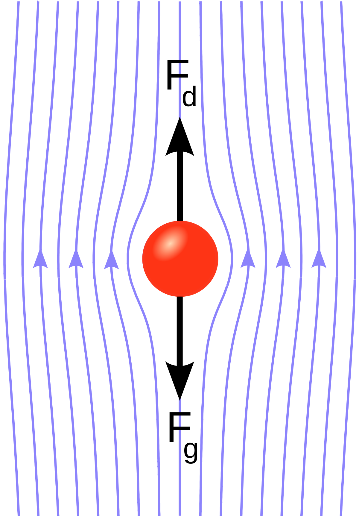
Consider a sphere of density $\rho_s$ and fluid of density $\rho_f$. The viscosity is given by $\nu = \rho_f \eta$. The Stoke’s Law gives us the drag force in terms of these parameters:

$$F_\text{drag} = 6\pi \eta v a$$

In a gravitational field $\vec g$, a falling sphere can reach terminal velocity. The terminal speed is:

$$v_\text{terminal} = \frac{2}{9}\frac{ga^2}{\nu}\left(\frac{\rho_s}{\rho_f}-1\right)$$

We can also show that:

$$\nabla^2 P = 0$$

and

$$\nabla^2 \vec \omega = \nabla^2(\vec \nabla \times \vec v)= 0$$

An Aisde

Millikan had oil dropping in air, allowing the oil to fall between two metal plates. We can reach the terminal velocity with the oil, and the electric field will accelerate the oil drops upward. By applying a known $\vec E$, Millikan can calculate the electric charge-to-mass ratio of the electron!

Accretion Disks

Astrophysical disks are ubiquitous. This is primarily because of angular momentum. The locations of these disks can be found:

• around planets

• around stars

• around black holes

• around neutron stars

When accreted gas has a non-zero $\vec L$, it generally forms an accretion disk. How does the gas inside this disk redistribute itself? If the gas loses angular momentum, the gas migrates inward. We can lose angular momentum via, for example, radiating energy away with photons, viscous torques, etc.

The goal of today is to get to the time-evolution equation for a flattened, idealized, axisymmetric disk. How does a ring of gas evolve in the presence of viscosity?

Consider an axisymmetric, thin disk (i.e., symmetry about $\varphi$). We will use cylindrical coordinates, with $\hat z$ out of the disk plane. The disk rotation is thus: $\vec \Omega = \Omega \hat{z}$. Axisymmetry tells us that:

$$\partial_\varphi \left(\text{anything}\right) = 0$$

We will also ignore the vertical spread (i.e., we have a razor thin disk) (we can thus ignore $v_z$). We are intersted in:

$$\vec v = v_\varphi \hat{\varphi} + v_R \hat{R}$$

The orbital motion is $v_\varphi$ and the radial motion is $v_R$, but subject to viscous forces, do these to decay?

We will also asssume that the central object (whatever it may be) is already in place, and thus we can ignore self-gravity.

Solving the problem…

Continuity

Let’s start with the continuity equation. We did this before for a disk, and we get:

$$\frac{\partial \rho}{\partial t} + \vec \nabla (\rho \vec v) = 0 \rightarrow \frac{\partial \Sigma}{\partial t} + \vec \nabla (\Sigma \vec v) = 0$$

Where $\Sigma = \int \rho dz$.

We can show that:

$$\boxed{\frac{\partial \Sigma}{\partial t} + \frac{1}{R}\frac{\partial}{\partial R} (\Sigma R v_R) = 0 }$$

We want to know a few things:

• Inward mass accretion rate (across R) of a ring at distance $R$ onto central object

The mass of this ring is $\Delta M = \rho 2\pi R \Delta R \Delta z$. The mass rate moving across $R$ is thus:

$$\frac{\Delta M}{\Delta t} = \rho \cdot 2\pi R \underbrace{\frac{\Delta R}{\Delta T}}_{v_R}\Delta z$$

And so:

$$\dot{M} = - \int \rho \cdot 2\pi R v_r \cdot dz$$

And we know that $\rho \cdot dz$ is just $\Sigma$, so:

$$\boxed{\dot{M} = - 2\pi R \Sigma v_R}$$

Note that we have chosen our sign such that $\dot{M} > 0$ for inflow (the $v_R$ is less than $0$). Thus all the action is going to be solving for $v_R$!

Momentum Equation (Navier-Stokes Equation)

Recall the Navier-Stokes equation:

$$\underbrace{\frac{\partial \vec v}{\partial t}}_{0 \text{ bc const. flow} } + (\vec v \cdot \vec \nabla) \vec v = -\frac{1}{\rho} \vec \nabla P - \underbrace{\vec \nabla \Phi}_\text{ignore for now} + \nu\left(\nabla^2 \vec v+ \frac13 \vec \nabla (\underbrace{\vec \nabla \cdot \vec v}_\text{0 bc incompressible})\right)$$

The key portion of this is the $\varphi$ component.

We know $\partial_\varphi P = 0$ due to axisymmetry. We skip a bunch of tedious math here….and just quote the result:

$$\boxed{ \Sigma \frac{\partial v_\varphi}{\partial t} + \Sigma \frac{V_R}{R} \frac{\partial }{\partial R}\left(R v_\varphi\right) = \frac{\partial}{\partial R} \left(\Sigma \nu \frac{\partial v_\varphi}{\partial R}\right) + \frac{1}{R} \frac{\partial}{\partial R}\left(\Sigma \nu v_\varphi\right) - \Sigma \nu \frac{v_\varphi}{R^2}}$$

We want to combine this equation above with the mass conservation equation we boxed above! To do this,

• Take $1 \times R v_\varphi + 2\times R$. where $1$ is the top equation and $2$ is the bottom equation.

All together, combining all our terms, we get a key equation:

$$\frac{\partial}{\partial t}\left(\Sigma R^2 \Omega\right) + \frac{1}{R} \frac{\partial}{\partial R} \left(\Sigma R^3 \Omega v_R\right) = \frac{1}{R}\frac{\partial}{\partial R} \left(\nu \Sigma R^3 \frac{\partial \Omega}{\partial R}\right)$$

We will call this equation $3$.

• It looks scary, but let’s examine this. Recall that $v_\varphi = R \Omega$. Recognizing this fact, the first term is simply the Eulerian rate of change of the angular momentum of an annulus of gas at radius $R$ (per unit area). This is basically just a conservation of angular momentum equation!

• The second term is just the net rate of angular momentum loss from this unit area due to advection of $L$ with radial flow.

• The right-hand side is the source term. This is the net viscous torque exerted on the annulus.

Why is the right hand side a torque? Let’s examine this a bit more. We can say:

$$\frac{1}{R}\frac{\partial}{\partial R} \left(\nu \Sigma R^3 \frac{\partial \Omega}{\partial R}\right) \equiv \frac{1}{2\pi R}\frac{\partial T}{\partial R}$$

where

$$T \equiv 2\pi \nu \Sigma R^3 \frac{\partial \Omega}{\partial R}$$

Note that $T<0$ is $\frac{d\Omega}{dR} < 0$. And also note that $T=0$ if we have rigid body rotation ($\frac{\partial \Omega}{\partial R} = 0$). The torque thus comes from particles traveling with viscosity (differential rotation).

• For most reasonable mass profiles, $\frac{\partial \Omega}{\partial R} < 0$. The inner parts are faster than the outer parts! Thus the inner gas moves faster (angularly) than outer gas. Viscosity exerts a negative torque $T$, slowing it down.

We need a bit more massaging of our equations to get an expression for $\partial_t \Sigma$. Here, we combine equations $1$ and $3$. We also assume that $\dot{\Omega} = 0$. We can take $3 \times R - 1 \times R^3 \Omega$. Doing this to our equations, we get a very general equation:

$$\boxed{\frac{\partial \Sigma}{\partial t} = - \frac{1}{2\pi R} \frac{\partial}{\partial R} \left(\frac{1}{\left(R^2 \Omega\right)^\prime }\frac{\partial T}{\partial R}\right)}$$

where

$$(R^2 \Omega)^\prime \equiv \frac{\partial }{\partial R}(R^2 \Omega)$$

is just a shorthand.

Let’s take the equation above and look at a Keplerian disk case (central point source). In this case, we have: $v_\varphi = R\Omega$ by definition. This is also:

$$v_\varphi = R\Omega = \sqrt{\frac{GM}{R}}$$

$\Omega$ in our case is:

$$\Omega = A R^{-3/2}$$

for Keplerian orbits, where $A$ is just some amplitude. This means that $(R^2 \Omega)^\prime = \frac{A}{2}R^{-1/2}$. The torque term becomes:

$$T = 2\pi \nu \Sigma R^3 \frac{\partial \Omega}{\partial R} = -3\pi\nu\Sigma R^3 \cdot \left(AR\right)^{-5/2}$$

We can now calculate $\partial T / \partial R$, and we get:

$$\frac{1}{(R^2 \Omega)^\prime} \frac{\partial T}{\partial R} = -6\pi R^{1/2} \frac{\partial}{\partial R}(\nu \Sigma R^{1/2})$$

And we get our final equation:

$$\boxed{\frac{\partial \Sigma}{\partial t} = \frac{3}{R}\frac{\partial}{\partial R}\left(R^{1/2} \frac{\partial}{\partial R} \left(\nu \Sigma R^{1/2}\right)\right)}$$

This is the basic equation for the time-evolution of surface density in a Keplerian accretion disk!!

---

We continue here from last time, where we considered a Keplerian disk. By combining the continuity equatio and the Navier-Stokes equation, we found that, assuming Keplerian rotation, the surface mass density evolves according to:

$$\frac{\partial \Sigma(R,t)}{\partial t} = \frac{3}{R}\frac{\partial}{\partial R}\left(R^{1/2} \frac{\partial}{\partial R} \left(\nu \Sigma R^{1/2}\right)\right)$$

This equation has solutions which we will see in Problem Set 6. We assume that the solution is separable.

For an initial delta function surface-density at $R=R_0$ (a ring):

$$\Sigma(R,t=0) = \frac{m }{2\pi R_0}\delta(R-R_0)$$

One can show that:

$$\boxed{\Sigma(R,t) \rightarrow \Sigma(x,\tau) = \frac{m}{\pi R_0^2} \frac{1}{\tau x^{1/4}} e^{-\frac{1+x^2}{\tau}} I_{1/4}\left(\frac{2x}{\tau}\right)}$$

where the dimensionless quantities are defined as $x \equiv R/R_0$ and $\tau = \frac{12\nu t}{R_0^2}$ and where $I_{1/4}$ is the modified Bessel function of order 1/4. What does this equation mean?

If we combine the continuity equation with the equation above, we can show that:

$$v_R = -\frac{3\nu}{R_0} \frac{\partial}{\partial x} \left(\frac14 \ln x + \frac{1+x^2}{\tau} + \ln I_{1/4}(\frac{2x}{\tau})\right)$$

We now want to see what $v_R$ is close and far from our source. Note that:

$$I_{1/4}(z) \propto z^{-1/2} e^{z} \text{ for } z \gg 1$$

$$I_{1/4}(z) \propto z^{1/4} \text{ for } z \ll 1$$

For $2x\gg \tau$: the right side is positive if and only if $x>1$ (beyond the ring):

$$v_{R} \approx \frac{3 \nu}{R_{0}}\left[\frac{1}{4 x}+\frac{2 x}{\tau}-\frac{2}{\tau}\right]$$

Thus for $R>R_0$, mass flows to larger radii, taking angular momentum away.

For $2x \ll \tau$:

$$v_{R} \approx-\frac{3 \nu}{R_{0}}\left[\frac{1}{2 x}-\frac{2 x}{\tau}\right]$$

Thus $v_r < 0$ if $\tau > 4x^2$. The implication is that the inner portion of the disk (satisfying this condition) moves inward.

Sources of Viscosity

• We still haven’t said anything about $\nu$ other than that it is a parameter. Which is faster, though – the processes that govern accretion or the processes that govern viscosity?

The most natural question one can ask is thus: what is the associated timescale of molecular viscosity?

• Inward velocity:

$$v_R \sim -\frac{3\nu}{R_0}\frac{1}{2x} \sim -\frac{3}{2}\frac{\nu}{R_0}$$

The timescale of radial inflow is thus:

$$t_{inflow} \sim \frac{R}{|v_R|} \sim \frac{R^2}{\nu} \sim \underbrace{\frac{R}{v_\varphi}}_\text{orbital timescale} \underbrace{\frac{R v_\phi}{\nu}}_\text{Reynold's number!}$$

$$t_{inflow} \sim \mathcal{R} t_{orbital}$$

Orbital times are quite fast – all that matters is our Reynold’s number! So what are relevant Reynold’s number for astrophysical accretion disks?

Well, recall that:

$$\nu \sim v_{thermal} \cdot \ell_{mfp} \sim v_{th} \frac{1}{\sigma n} \rightarrow \mathcal{R} \sim \frac{R v_\varphi}{v_{thermal} \ell_{mfp}} \sim \frac{R v_\varphi}{v_{th}} \sigma n$$

In a typical region of an astrophysical accretion disk around a star:

• $R \sim 10^{10} \text{ cm}$

• $T_{gas} \sim 10^4 \text{ K}$, anything hotter becomes warm/hot x-ray gas. Anything lower is molecular clouds. This is about right for a hydrogen/helium disk. We have $k_b T \sim \frac12 mv^2 \rightarrow v_{th} \sim 10 \text{ km } \text{ s }^{-1}$.

• $n \gtrsim 10^{15} \text{ cm}^{-3}$

• $\sigma \sim 10^{-16} \text{ cm}^2$

• $v_\phi \sim 100 \text{ km } \text { s }^{-1}$

This gives:

$$\nu \sim \frac{v_{th}}{\sigma n} \sim 10^7 \frac{\text{cm}^2}{\text{s}}$$

We also had:

$$v_R \sim \frac{\nu}{R} \sim \frac{10^{7}}{10^{10}} \sim 10^{-3} \frac{\text{cm}^2}{\text{s}} \ll v_\varphi$$

And what is the Reynold’s number here?

$$\boxed{\mathcal{R} \sim \frac{R v_\varphi}{\nu} \sim 10^{10}}$$

Thus:

$$\boxed{t_{inflow} \sim 10^{10} t_{orb} \gg t_\text{Hubble}}$$

So what does this mean? It means that molecular viscosity alone is simply not effective at bringing material toward the central object. So what other processes could dominate the inflow?

previous

Fluid Instabilities

next

Kinetic Theory