.md .pdf

repository open issue

Contents

Fluid Instabilities

Gravitational Instabilities in a Static vs. Expanding Medium

Let’s recall two of the dispersion relations we have derived:

Free Wave Dispersion Relation: Sound Waves

$$\omega = v_s k$$

Surface Water Waves

Here, we had gravity (constant), which gives a dispersive relation:

$$\omega^2 = gk\tanh(kH)$$

where $H$ is the depth of the sea. Also note that here, we had $\vec \nabla \Phi = -\vec g$.

And also, recall our equations for linear perturbation theory:

$$\rho = \rho_0 + \rho_1$$

$$P = P_0 + P_1$$

$$\vec v = \vec v_0 + \vec v_1$$

$$\Phi = \Phi_0 + \Phi_1$$

Note that $\rho_1 \ll \rho_0$, and so forth. We also had things like the adiabatic sound speed:

$$v_s^2 = \left(\frac{\partial P}{\partial \rho}\right)_\text{const. S} = \frac{P_1}{\rho_1}$$

Static, Uniform Medium

For a static, uniform medium, we have $\rho_0 = \text{const.}$, $P_0 = \text{constant}$, and $\vec v_0 = 0$. The potential is interesting, though, which we will return to. The fluid equations are:

Zeroth Order Continuity Equation

$$\frac{\partial \rho_0}{\partial t} + \vec \nabla (\rho_0 \vec v_0) = 0$$

This is trivially true.

Zeroth Order Euler Equation

The LHS is $0$ since $\vec v_0 = 0$. The RHS of the Euler equation tells us that:

$$-\frac{1}{\rho_0} \vec \nabla P_0 - \vec \nabla \Phi_0 = 0 \rightarrow \vec \nabla \Phi_0 = 0$$

Zeroth Poisson Equation

We have:

$$\nabla^2 \Phi_0 = 4\pi G \rho_0$$

Since we are radially symmetric, we have:

$$\vec \nabla \Phi_0 = \frac{4\pi}{3} G\rho_0 \vec{r}$$

Hey! Wait a minute! The two zeroth order equations tell us that $\rho_0$ has to be 0. This isconsistency is actually called the Jeans-Swindle. The reason we have an inconsistency is because we need our medium to be infinitely large. Thus, the Jean’s Swindle is a reflection of the unrealistic background we are considering.

We now go to the perturbed equations:

First Order Continuity

$$\frac{\partial \rho_1}{\partial t} + \rho_0 \vec \nabla \cdot \vec v = 0$$

First Order Euler

$$\frac{\partial \vec v_1}{ \partial t} = - \frac{v_s^2}{\rho_0} \vec \nabla P_1 - \vec \nabla \Phi_1$$

First Order Poisson

$$\nabla^2 \Phi_1 = 4\pi G \rho_1$$

We can combine the first two equations, taking the time derivative of the first. Doing so, we get:

$$\frac{\partial^2 \rho_1 }{\partial t^2} + \rho_0 \left(-\frac{v_s^2}{\rho_0} \nabla^2 \rho_1 - \nabla^2 \Phi_1\right) = 0$$

Now use the Poisson equation (equation 3), to give a wave’s equation with a driving term:

$$\boxed{\frac{\partial^2 \rho_1}{\partial t^2} - v_s^2 \nabla^2 \rho_1 - 4\pi G\rho_0 \rho_1 = 0}$$

We use Fourier analysis, turning a differential into algebraic equation, since the modes decouple. We do this by saying $\rho(\vec r, t) \propto \int e^{i (\vec k \cdot \vec r - \omega t)} \, c(\vec{k}) \, d^3 k$ . However, if we had non-linear terms like $\rho_1^2$, all Hell breaks loose in Fourier space. This is because we have convolutions when things are non-linear, and that is ugly.

Anyways, we get:

$$-\omega^2 + v_s^2 k^2 - 4\pi G\rho_0 = 0$$

Dispersion Relation for Jean’s Instability

$$\boxed{\omega^2 = v_s^2 k^2 - 4\pi G \rho_0}$$

This is a dispersive wave (since we are non-linear in $k$). We can also immediately see that $\omega$ might be imaginary! If pressure wins, we have waves/oscillatory behavior! If gravity wins, we get exponential collapse.

We can write this in a bit different way:

$$\omega^2 = v_s^2 \left(k^2 - k_J^2\right)$$

where:

$$k_J \equiv \sqrt{\frac{4\pi G \rho_0}{v_s^2}}$$

is the Jean’s wavenumber. We also often see:

$$\lambda_J \equiv \frac{2\pi}{k_J}$$

And Jean’s mass (the mass enclosed within $\lambda_J$):

$$M_J = \frac{4\pi}{3} \lambda_J^3 \rho_0$$

And we often say things like ``what is the Jean’s mass/Jean’s length at a time in cosmic history?’’ Here, we compare the density to the sound speed, more or less, through the definition of Jean’s wavenumber.

Note that pre-CMB, the Jean’s Length is huge. After free electrons combine with ionized hydrogen (forming neutral hydrogen), photons free stream. Thus, the Jean’s Mass drops tremendously. The Jean’s Mass post-recombination is of order $10^{6}$ solar masses. This is when structure formation takes off!

Two Regimes

Regime A

We consider here $k > k_J$ or $\lambda < \lambda_J$. In this case, we have $\omega^2 > 0$, and thus $\omega$ is real. $\rho_1$ oscillates like sound waves. This is a stable solution.

Regime B

Here $\omega^2<0$, and thus $\omega$ is imaginary. This implies:

$$\rho_1 \propto e^{\pm |\omega| t}$$

The growing solution is exponential!

An Side

Note that the dispersion relation for Jean’s instability is very similar to the plasma frequency:

$$\omega^2 = v_s^2 k^2 + \frac{4\pi n_e e^2}{m_e} > 0$$

Thus the plasma frequency is always oscillatory!

An Expanding Medium

In this case, we have:

$$\rho_0 = \rho_0(t)$$

We can define a $\delta$ such that:

$$\delta \equiv \frac{\rho_1}{\rho_0} = \frac{\rho - \rho_0}{\rho_0} = \left(\delta \rho\right)$$

The overdensity can be as large as can be, but the underdensity can only get as negative as $-1$. This negative overdensity regions of the Universe are called voids. Thus $(-1 \leq \delta < \infty)$.

Also note that our fluid velocity is no longer $0$. Instead, we have $\vec v_0 = H \vec r$ (Hubble expansion). This is also $\vec v = \frac{\dot{a}}{a}\vec r$. By convection, we choose $a=1$ today, and $a<1$ before today. Note that taking:

$$\vec \nabla \cdot \vec v_0 = 3 \frac{\dot{a}}{a}$$

And note that

$$\vec{v}_1 = \text{ peculiar velocity}$$

We now go to our fluid equations:

Zeroth Order Continuity

$$\frac{\partial \rho_0}{\partial t} + \rho_0 \vec \nabla \cdot \vec v_0 = \frac{\partial \rho_0}{\partial t} + \frac{3\dot{a}}{a} \rho_0 = 0 \rightarrow \rho_0(t) \propto \frac{1}{a(t)^3} \propto \frac{1}{\text{volume}}$$

This is nice and in accordance with our intuition.

First Order Continuity

$$\frac{\partial \rho_1}{\partial t} + \rho_0 \vec \nabla \cdot \vec v + \vec \nabla (\rho_1 \vec v) = 0$$

We’ll now want to go to $\delta$ coordinates in our first order continuity equation:

$$\rho_1 = \rho_0 \delta \rightarrow \rho_0 \dot{\delta} +\delta \dot{\rho}_0 + \rho_0 \vec \nabla \cdot \vec v_1 + \rho_0 \vec v_0 \cdot \vec \nabla \delta + \rho_0 \delta \vec \nabla \cdot \vec v = 0$$

Also note that $\dot{\rho}_0 = -3\frac{\dot{a}}{a}$ from the continuity equation, and we know that $\vec \nabla \cdot \vec v_0 = 3\frac{\dot{a}}{a}$. This cancels nicely:

Dividing through by $\rho_0$, we get the linearized Continuity Equation for an expanding Universe:

$$\dot \delta + \vec \nabla \cdot \vec v_1 + \frac{\dot a}{a} \vec r\cdot \vec \nabla \delta = 0$$

where we have replace $v_0$ with Hubble’s Law.

Zeroth Order Euler Equation

Again, $\vec v_0$ is not zero, and so we just get a constra:

$$\frac{\partital \vec v_0}{\partial t} + (\vec v_) \cdot \vec \nabla) \vec v_0 = - \vec \nabla \Phi_0$$

First Order Euler Equation

$$\frac{\partial \vec v_1}{\partial t} + (\vec v_0 \cdot \vec \nabla) + (\vec v_1 \cdot \vec \nabla) \vec v_0 = -\frac{v_s^2}{\rho_0} \vec \nabla \rho_1 - \vec \nabla \Phi_1$$

Let’s simplify the ugly term:

$$(\vec v_1 \cdot \vec \nabla) \vec v_0 = \frac{\dot a}{a} (\vec v_1 \cdot \vec \nabla) \vec r$$

And note that:

$$\vec v_1 \cdot \vec \nabla = v_{1x} \partial_x + v_{1y} \partial_y + v_{1z} \partial_z$$

And so acting on $\vec{r}$, we get: $(\vec v_1 \cdot \vec \nabla) \vec r = \frac{\dot a}{a} \vec{v}_1$.

This makes our First Order Euler equation;

$$\frac{\partial v_1}{\partial t} + \frac{\dot{a}}{a}(\vec r \cdot \vec \nabla) \vec v_1 + \frac{\dot a}{a} \vec v_1 = -v_s^2 \vec \nabla \delta - \vec \nabla \Phi_1$$

And finally, our Poisson:

Zeroth and First Order Poission

We get:

$$\nabla^2 \Phi_0 = 4\pi G \rho_0$$

$$\nabla^2 \Phi_1 = 4\pi G \rho_0 \delta$$

We no longer have Jean’s Swingle, by the way!

---

Here, we continue from last week. Let’s recall a few things:

Static Case: Pressure vs. Gravity

In this case, we derived:

$$\omega^2 = v_s^2 k ^2 - 4\pi G \rho_0$$

or

$$\omega^2 = v_s^2 \left(k^2 - k_J^2\right)$$

where $k_J$ is the Jeans Wavenumber, defined as:

$$k_J \equiv \sqrt{\frac{4\pi G\rho_0}{v_s^2}}$$

We got this by perturbing our fluid equations in the limit where the sub-0 pieces do not depend on time, nor space. We then moved into the contracting or expanding medium.

Expanding Case

The linearized fluid equations were dervied last time. These were:

From the continuity equation: $$\dot{\delta} + \vec \nabla \cdot \vec v_1 + \frac{\dot a}{a}\left(\vec r \cdot \vec \nabla\right) \delta = 0$$

From the Euler equation:

$$\frac{\partial \vec v_1}{\partial t} + \frac{\dot a}{a}\left(\vec r \cdot \vec \nabla\right)\vec v_1 + \frac{\dot a}{a} \vec v_1 = -v_s^2 \vec \nabla \delta - \vec \nabla \Phi$$

Note that we might have had this expression wrong last time. We had an extra $\rho_0$ somewhere.

And from the Poisson equation:

$$\nabla^2 \Phi_1 = 4\pi G \rho_0 \delta$$

To solve these equations, we go into Fourier space. Also, we will go into the co-moving coordinate system which will cancel out many of the terms. First, doing the Fourier Transform:

To go to co-moving coordinates:

$$\vec r = a(t) \vec x$$

where $\vec r$ is physical and $\vec x$ are the co-moving coordinates. Note that $a(\text{today}) = 1$. Correpsondingly, our co-moving wave number $\vec k$ will be paried with $\vec x$ and not $\vec r$. Go to Fourier Space:

$$\delta(\vec r, t)$$

$$\vec v_1 (\vec r, t)$$

$$\Phi_1(\vec r, t)$$

These three quanities are:

$$= \int \mathrm{d}^3 \, k \, e^{i\frac{\vec k \cdot \vec r}{a(t)}} f_k(t)$$

where $f_k(t)$ are the Fourier transformed functions. In one shot, we will do a lot of algebra here. We will calculate $\dot{\delta}$ in real space:

$$\dot \delta(\vec r, t) = \int d^3\,k\, e^{i\frac{\vec k \cdot \vec r}{a(t)}} \left(\dot{\delta}_k - \frac{\dot a}{a} i \frac{\vec k \cdot \vec r}{a(t)} \delta_k\right)$$

And

$$\vec \nabla \delta(\vec r, t) = \cdots \frac{i \vec k}{a(t)}\delta_k$$

And

$$\vec \nabla \cdot \vec v_1(\vec r,t) = \cdots i \frac{\vec k}{a}\vec v_k$$

Now, with these, our CONTINUITY EQUATION becomes:

$$\dot{\delta}_k - \frac{\dot a}{a} \frac{i \vec k \cdot \vec r}{a} \delta_k + i \frac{\vec k \cdot \vec v_k}{a} + \frac{\dot a}{a} \left(\vec r \cdot i \frac{\vec{k}}{a}\right)\delta_k = 0$$

We get cancellations, and thus:

$$\boxed{\dot \delta_k + i \frac{\vec k \cdot \vec v_k}{a} = 0}$$

Our Euler equation is:

$$\dot{\vec v}_k - \frac{\dot a}{a} i \frac{\vec k \cdot \vec r}{a}\vec v_k + \frac{\dot a}{a}\left(\vec r \cdot \frac{i \vec k}{a}\right)\vec v_k + \frac{\dot a}{a}\vec v_k = -v_s^2 \frac{i \vec k}{a}\delta_k - i\frac{\vec k}{a}\Phi_k$$

We get cancellations and combinations (with total derivatives), giving the linearized euler equation!

$$\boxed{\frac{\partial}{\partial t} \left(a \vec v_k\right) + i v_s^2 \vec k \delta_k + i \vec k \Phi_k = 0}$$

And our Poisson equation:

$$\boxed{\frac{k^2}{a^2} \Phi_k = - 4\pi G \rho_0 \delta_k}$$

And we now combine our three boxed equations in the most efficient way possible for an equation for $\delta$. How do we do that?

1. We begin by getting rid of $\vec v$. We do this by multiplying our first equation by $a^2$. Doing so, this becomes:

$$a^2 \dot{\delta}_k + i \vec k \cdot \left(a \vec v_k\right) = 0$$

2. And we now take $\partial_t$, and use the second equation to replace the first term. This gives, using the second equation above:

$$a^2 \ddot{\delta}_k + 2a \dot{a} \dot{\delta}_k + i \vec k \cdot (-i v_s^2 \vec k \delta_k - i \vec k \Phi_k) = 0$$

3. Divide by $a^2$:

$$\ddot{\delta}_k + 2 \frac{\dot{a}}{a}\dot{\delta}_k + \frac{v_s^2 k^2}{a^2} \delta_k - \underbrace{4\pi G \rho_0 \delta_k}_\text{using Poisson from above} = 0$$

And now we have one equation!

$$\boxed{\ddot{\delta}_k + 2\frac{\dot a}{a} \dot{\delta}_k + \frac{v_s^2}{a^2}\left(k^2 - k_J^2\right)\delta_k = 0}$$

where

$$\boxed{k_J^2 \equiv \frac{4\pi G \rho_0 a^2}{v_s^2}}$$

Note that this is the co-moving Jeans wavenumber, and since $\vec r = a \vec x$, the $a$ cancels out in the physical Jeans wavenumber. The key difference in the above equation is the $\dot{a}/a$ term, by the way, which makes sense for our intuition. Let’s look at some regimes.

Examine k < k_J regime:

In this case, we have:

$$\ddot{\delta}_k + 2\frac{\dot a}{a} \dot{\delta}_k - 4\pi G \rho_0 \delta_k = 0$$

In order to go further, we need to specify our Universe. The simplest case is a flat Universe (Einstein-de Sitter) model. In this case, $\Omega_{m} = 1$ (non-relativistic matter, no curvature, no Cosmological Constant, etc). Recall (or derive), and remember that $a \propto t^{2/3}$ for EdS Universe:

$$4\pi G \rho = \frac32 H^2(t) = \frac{\dot{a}^2}{a^2} = \frac{2}{3t^2}$$

And lastly, our equation for $\ddot{\delta}$ is:

$$\ddot{\delta}_k + \frac{4}{3t} \dot{\delta}_k - \frac{2}{3t^2} \delta_k = 0$$

Our Ansatz is: $\delta_k \propto t^{\alpha}$. This makes our expression:

$$\alpha(\alpha-1) + \frac43 \alpha - \frac23 = 0 \rightarrow \alpha^2 + \frac{\alpha}{3} = \frac23$$

$$(\alpha -\frac23)(\alpha+1) = 0 \rightarrow \boxed{\alpha = \frac23 , -1}$$

What did we find here? We found that $\delta \propto t^{2/3} \propto a$ or $\delta \propto t^{-1}$. These represents the growing and decaying mode respectively. We can compare these with the static Universe, in which $\delta$ is exponential $\propto e^{\pm \omega t}$, and not a power law. The thing that slows the exponential growth is the drag term due to the expansion of the Universe.

The expansion slows to a power-law form, from an exponential form in the static case. All these different modes, by the way, decouple and have the same behavior. Density perturbations grow like the scale factor in the flat Universe case.

Take a look into the dark matter power spectrum, by the way! We derived the time-growth of the power spectrum! The power spectrum of dark matter grows with $a^2$.

Note that we only solved these expressions for the pertubration growth, but we can do the same with the $\vec v$ and $\Phi$.

Gravitational Instability of a Rotating (Self-Gravitating) Disk

Consider a uniformly rotating sheet of zero thickness with constant angular velocity $\vec \Omega = \Omega \hat{z}$. We assume a constant surface density $\Sigma_0$. We also assume the sheet is in the $(x,y)$ plane at $z=0$. Usually, it’s easier to go into the moving frame. Thus, we go into the rotating frame.

In the frame that rotates with the unperturbed sheet, consider small perturbations in the $(x,y)$ plane.

$$\Sigma(x,y,t) = \Sigma_0 + \Sigma_1 (x,y,t)$$

And note that our 3D density, knowing that our disk is razor thin, is:

$$\rho = \Sigma \cdot \delta(z)$$

We have a fluid moving in the disk with velocity:

$$\vec v(x,y,t) = \vec v_0 + \vec v_1(x,y,t)$$

In the rotating frame, $\vec v_0 = 0$, and thus:

$$\vec v(x,y,t) = \vec v_1(x,y,t)$$

As a consequence of going into the rotating frame, we will have to deal with fictitious forces later.

Our pressure is:

$$P(x,y,t) = P_0 + P_1(x,y,t)$$

Note that, because we are in 2D, our sound speed is defined a bit differently, such that:

$$v_s^2 = \frac{\partial P}{\partial \Sigma} = \frac{P_1}{\Sigma_1}$$

Which is a statement saying that pressure acts only in the plane, and not upward or donward.

And potential:

$$\Phi(x,y,t) = \Phi_0 + \Phi_1(x,y,t)$$

The fluid equations take the following form.

Continuity in 2javascript

\frac{\partial \Sigma}{\partial t} + \vec \nabla (\Sigma \vec v)= 0 \rightarrow \text{ Perturbed } \rightarrow \boxed{\frac{\partial \Sigma_1}{\partial t} + \Sigma_0 \vec \nabla \cdot \vec v = 0 }

Euler Equation

$$\frac{\partial \vec v}{\partial t} + (\vec v \cdot \vec \nabla) \vec v = -\frac{1}{\Sigma} \vec \nabla P - \vec \Phi \underbrace{- 2\vec \Omega \times \vec v}_\text{Coriolis} + \underbrace{\Omega^2 \left(x\hat{x} + y\hat{y}\right)}_\text{centrifugal force}$$

Note that this is where we have to pay the price of going to the rotating frame. Those extra terms might look ugly, but they’re not all that bad.

We can write down our perturbed pieces:

$$\boxed{\frac{\partial \vec v_1}{\partial t} = -\frac{v_s^2}{\Sigma_0} \vec \nabla \Sigma_1 - \vec \nabla \Phi_1 - 2\vec \Omega \times \vec v}$$

Poisson

$$\nabla^2 \Phi = 4\pi G \Sigma \delta(z)$$

Perturbing this, we find:

$$\boxed{\nabla^2 \Phi_1 = 4\pi G \Sigma_1 \delta(z)}$$

Note that the boxed equations are the perturbed equations. This is pretty similar to what we had before, but we have a nasty coriolis term which prevents our usual tricks.

---

Let’s continue. Recall from last time that:

$$\frac{\partial \Sigma_1}{\partial t} + \Sigma_0 \vec \nabla \cdot \vec v_1 = 0$$

$$\frac{\partial \vec v_1}{\partial t} = - \frac{v_s^2}{\Sigma_0}\vec \nabla \Sigma_0 - \vec \nabla \Phi_1 - 2\vec \Omega \times \vec v_1$$

$$\nabla^2 \Phi_1 = 4\pi G \Sigma_1 \delta(z)$$

from the Continuity equation, Euler’s equation, and Poisson equation, respectively. The coriolis force restricts us from doing our normal trick. Still, though, we will do a Fourier Transform since we have linearized equations. In this case, we have $(x,y)\rightarrow(k_x,k_y)$. But, we can choose our orientation such that $\vec k = k \hat{x}$, i.e., $k_y = k_z = 0$. Additionally, we have: $\vec k \cdot \vec r = kx$.

Doing so:

$$\Sigma_1(x,y,t) = \int d^3\,k \Sigma_1(k) e^{i(kx-\omega t)}$$

And the same form for velocities $v_{1x}$ and $v_{1y}$:

$$v_{1x}(x,y,t) = \int \, d^3\,k v_{1x}(k) e^{i(kx-\omega t)}$$

$$v_{1y}(x,y,t) = \int \, d^3\,k v_{1y}(k) e^{i(kx-\omega t)}$$

$$\Phi_1(x,y,t) = \int \, d^3\,k \Phi_{1}(k) e^{i(kx-\omega t)} \text{ at z=0}$$

$$\Phi_1(x,y,z,t) = \int \, d^3\,k \Phi_{1}(k) e^{i(\vec k \cdot \vec r-\omega t)} \text{ at z not 0}$$

We will start with the Poisson equation first, keeping in mind it depends on where in $z$ we are:

At $z=0$, we have:

$$\nabla^2 \Phi_1 = 4\pi G \Sigma_1$$

At $z\neq 0$:

$$\nabla^2 \Phi_1 = 0$$

This is the Laplace equation, which we have solved before when solving for water waves. For $z\neq 0$, that is – above or below the plane – we have:

$$\Phi_1 (x,y,z,t) \propto e^{i(kx-\omega t)} \mathcal{f}(z) \Phi_1(k)$$

Recall that the vertical structure $\mathcal{f}(z)$, we had:

$$-k^2 \mathcal{f} + \frac{d^2 \mathcal{f}}{dz^2} = 0 \rightarrow \mathcal{f}(z) \propto e^{\pm kz}$$

To have $\mathcal{f}$ be $0$ at infinity, we need:

$$\mathcal{f} \propto e^{-k|z|}$$

For $z \approx 0$: we can integarte the Poisson equation from slightly below $-\epsilon$ to slightly above $+\epsilon$:

$$\lim_{\epsilon \rightarrow 0 } \int_{-\epsilon}^{\epsilon} \mathrm{d}z \, \frac{\partial^2 \Phi_1}{\partial z^2} = 4\pi G \Sigma_1 \underbrace{\int_{-\epsilon}^{\epsilon} \delta(z) \mathrm{d}\,z}_{=1}$$

And thus:

$$\lim_{\epsilon \rightarrow 0} \left(\frac{\partial \Phi_1}{\partial z} \Bigg\vert_{z=+\epsilon} - \frac{\partial \Phi_1}{\partial z} \Bigg\vert_{z=-\epsilon}\right) = 4\pi G\Sigma_1$$

We now go into $k$ space:

$$\lim_{\epsilon \rightarrow 0} \left(-ke^{-k|z|} \Phi_1\Big\vert_{z=+\epsilon} - k e^{k|z|}\Phi_1 \Big\vert_{z=-\epsilon}\right) = 4\pi G \Sigma_1$$

$$-2k \Phi_1 = 4\pi G \Sigma_1$$

We thus just showed that:

$$\boxed{\Phi_1 = -\frac{2\pi G}{k} \Sigma_1} \text{ in } k \text{ space}$$

We have used equation 3 from above to get this result. We now return to equations 1 and 2 from the Continuity and Euler’s equation.

From the first equation (continuity), we have:

$$- i \omega \Sigma_1 + \Sigma_0 i k v_{1x} = 0 \rightarrow \boxed{v_{1x} = \frac{\omega}{k}\frac{\Sigma_1}{\Sigma_0}}$$

From the Euler’s equation, let’s look at $\hat{y}$ first:

$$\hat{y}: -i\omega v_{1y} = -2(\vec \Omega \times \vec v_1)_{y} = -2\Omega v_{1x} \rightarrow v_{1y} = \frac{2\Omega}{i\omega} v_{1x}$$

Note that the $\Sigma_1$ and $\Phi_1$ terms vanished since we chose $\vec k = k \hat{x}$. Our Fourier Transform by choice has no y-dependence, so taking the gradient gives $0$ in non-x directions.

And now the $\hat{x}$ component:

$$\hat{x} : -i \omega v_{1x} = -\frac{v_s^2}{\Sigma_0} i k\Sigma_1 - ik\Phi_1 - \underbrace{2(\vec \Omega \times \vec v_1)_{x}}_{-\Omega v_{1y}}$$

Now, let’s combine our three linearized equations, getting rid of $\Phi_1$ and the $v$’s, writing in terms of $\Sigma_1$. We will start with the epxression for $\hat{x}$ direction:

$$-i \frac{\omega^2}{k}\frac{\Sigma_1}{\Sigma_0} = -\frac{ik v_s^2 \Sigma_1}{\Sigma_0} + i2\pi G \Sigma_1 + 2 \Omega (- i\frac{2\Omega}{k}\frac{\Sigma_1}{\Sigma_0})$$

Simplifying things a bit, we get:

$$\boxed{\omega^2 = v_s^2 k^2 - 2\pi G k \Sigma_0 + 4\Omega^2}$$

Dispersion Relation for Self-Gravitating, Rotating Disk

$$\omega^2 = \underbrace{v_s^2 k^2}_\text{pressure (stable)} - \underbrace{2\pi G k \Sigma_0}_\text{gravity (unstable)} + \underbrace{4\Omega^2}_\text{rotation (stable)}$$

Note that statements of stability are based on the sign of the term.

Let’s compare the above result with the spherical Jean’s dispersion relation:

$$\omega^2 = v_s^2 k^2 - 4\pi G\rho_0$$

Some Comments

If gravity dominates:

$$\omega^2 \approx -2 \pi G k \Sigma_0 < 0 \rightarrow \text{ always unstable}$$

Gravity and Pressure dominate ($\Omega \sim 0$):

$$\omega^2 = v_s^2 k^2 - 2\pi G k \Sigma_0 \rightarrow \omega^2 < 0 \text{ iff } \boxed{k<\frac{2\pi G\Sigma_0}{v_s^2} \equiv k_J}$$

Long-$\lambda$ perturbations are unstable.

Gravity and Rotation dominate ($v_s^2 \sim 0$):

$$\omega^2 < 0 \text{ iff } \boxed{k > \frac{2\Omega^2}{\pi G \Sigma_0}}$$

Hey! Look at that! The two regimes have different equality signs. In this case, short-$\lambda$ perturbations are unstable. This kinda of makes sense – its the overall rotation that stabilizes the system.

In general

Let’s complete the square

$$\omega^2 = v_s^2 \left(k - \frac{\pi G \Sigma_0}{v_s^2}\right)^2 + 4\Omega^2 - \left(\frac{\pi G \Sigma_0}{v_s}\right)^{2}$$

When do we have stable conditions? This is when $\omega > 0$ if:

$$2\Omega > \frac{\pi G \Sigma_0}{v_s}$$

Or, we can combine things:

$$\boxed{\frac{v_s \Omega}{G \Sigma_0} > \frac{\pi}{2} \sim 1.571}$$

Stability Criterion for Self-Gravitating Disk

$$\frac{v_s \Omega}{G \Sigma_0} > \frac{\pi}{2}$$

For a thin disk of (collisionless) stars rather than (collisional) fluid…

In this case, the sound speed $v_s$ is replaced by the characterstic speed of the stars (the velocity dispersion). In this case, we have a stable disk of stars if:

$$\boxed{\frac{\sigma \Omega}{G \Sigma_0} > 1.68}$$

for a Maxwellian velocity distribution of the stars.

This is the Toomre (1964) relation. Thus,

For a disk with a more realistic vertical structure (say, exponentially stratified instead of razor thin)

Then you can show that the gas disk is stable if:

$$\boxed{\frac{v_s \Omega}{G \Sigma_0} > 1.06}$$

This also assumes an isothermal equation of state.

For a differentially rotating disk of gas…

In this case, $\Omega$ is not a constant but has a radial profile $\Omega(R)$. Often, we replace $\Omega(R)$ with $\Omega$ with the epicycle frequency:

$$\kappa^2 = R \frac{\partial (\Omega)^2}{\partial R} + 4 \Omega^2$$

This makes the dispersion relation:

$$\omega^2 = k^2 v_s^2 - 2\pi G k \Sigma_0 + \kappa^2$$

And the disk is stable if:

Toomre Q Parameter

$$\boxed{Q \equiv \frac{v_s \kappa}{\pi G \Sigma_0} > 1 }$$

Note that we use $\sigma_R$ if we are talking about stars (radial velocity dispersion). Also note that we can teaase out a timescale, which is bascially the dynamical time. Think in terms of free-fall timescale.

This is called the Toomre’s Q parameter:

If you’re curious, check out Binney & Tremaine, Section 3.2. Epicycling is actually important in axisymmetric systems. This is because slightly elliptical orbits can be approximated as epicycling (to first-order Taylor expansions).

Examples of kappa:

$$\Omega(R) = \frac{V_{circ}(R)}{R} \rightarrow V_{circ} \equiv \sqrt{\frac{GM(<R)}{R}}$$

1. Point Mass:

Here, we have Keplerian orbits, and so:

$$V_{circ} \propto \sqrt{1/R} \rightarrow \Omega \propto R^{-3/2} \rightarrow \kappa^2 = \Omega^2$$

Thus, in the Keplerian case, there is just one frequency – the orbital frequency!

2. Flat Rotation Curves

For velocity to be constant, we need $M(<R)\propto R$, and thus $\rho \propto r^{-2}$. Note that $V_{c} = R \Omega \rightarrow \Omega \propto R^{-1}$, and finally, $\kappa = \sqrt{2}\Omega$.

3. Solid Body Rotation

Here, we have a rigid sheet with $\rho = \text{ constant}$. In this case, $M \propto R^{3}$ and $V_{c} \propto R$. This also makes $\Omega = \text{ constant}$, and we recover that $\kappa = 2\Omega$, which we started with.

Thus $\kappa$ ranges from roughly $\Omega$ to $2\Omega$ for reasonable galaxy shapes.

An Aside on the Jeans Instability

We are continuing from last time, and we are starting with a back of the envelope calculation for the Jean’s length. The key result is the dispersion relation:

$$\omega^2 = k^2 v_s^2 - 4\pi G \rho_0 = v_s^2 (k^2 - k_J^2)$$

Well, we know that:

$$k_J \equiv \sqrt{\frac{4\pi G\rho_0}{v_s^2}}$$

Dimensionally, we can do the same thing to tease out $G\rho / v_s^2$ dependence.

Back of the Envelope Analysis

The underyling physics is the balance of pressure and gravity. Let’s compare the forces, or more concretely, the timescale over which they act. Instability occurs if gravity wins over pressure.

1. Option 1: Comparing the Forces (per volume)

Consider a fluid of density $\rho$ , total mass $M$, and radius $R$. The fluid elements in this fluid has volume $V$. Thus:

$$\text{Gravity} \sim \frac{F_g}{V} \sim \frac{GM \rho}{r^2} \sim G\rho^2 R$$

Outward pressure is:

$$\text{Pressure} \sim \frac{F_p}{V} \sim \nabla P \sim v_s^2 \nabla \rho \sim \frac{v_s^2 \rho}{R}$$

Gravity wins if:

$$G \rho^2 R > \frac{v_s^2 \rho}{R} \rightarrow \boxed{R > \sqrt{\frac{v_s^2}{G \rho}}} \sim \lambda_J$$

2.Option 2: Comparing the Timescales

We have the timescale of gravity, the free-fall timescale, which is the time it takes to fall $R$:

$$R \sim a t_g^2 \sim \frac{GM}{R^2} t_g^2 \sim G\rho R t_g^2 \rightarrow t_g \sim \sqrt{\frac{R}{a}} \sim \boxed{\frac{1}{\sqrt{G\rho}}}$$

And the timescale for pressure is the sound-crossing time:

$$t_p \sim \frac{R}{v_s}$$

Gravity wins when $t_g < t_P$:

$$\frac{1}{\sqrt{G\rho}} < \frac{R}{v_s^2} \rightarrow R > \sqrt{\frac{v_s^2}{G\rho}}$$

which is exactly the same as we found above!

An Aside: The Coriolis Force

A quick physical insight! Recall that the Coriolis force is:

$$-2 \vec \Omega \times \vec v$$

Consider walking outward radially from a spinning disk and the forces!

Some final thoughts

We continue here from last time. Recall that, for a self-gravitating disk, we have:

$$\omega^2 = k^2 v_s^2 - 2\pi G k \Sigma_0 + 4 \Omega^2$$

Note that rotation and pressure are stabilizing, whereas gravity causes instabilities.

Rayleigh-Taylor Instability

This instability occurs when we have two fluids in a consatnt gravitational field $\vec{g}$. We will call the top fluid $\rho_+$ and the bottom fluid as $\rho_{-}$. What happens to perturbations traveling along the boundary?

Recall too that we defined $\xi_{z}$ which is a displacement of the perturbed fluid velocities.

In the top fluid, we have $\rho_+$, $v_+$, and $\vec v_+$. With subscript minus for the lower fluid. We begin with our zeroth order equations:

Zeroth Order Equations

In the single fluid case (surface water waves), we had:

$$\vec v_0 = 0$$

$$\frac{1}{\rho_0} \frac{\partial P_0}{\partial z} = - g$$

We found, for water waves, that:

$$P_0 = -\rho_0 g z + \mathcal{C}$$

We can easily generalize this to two fluids! In the top fluid, we will have:

$$P_{+0} = - \rho_{+0} g z + \mathcal{C}_{+}$$

In the bottom fluid, we have

$$P_{-0} = - \rho_{-0} g z + \mathcal{C}_{-}$$

Our first order equations are:

First Order Equations

For the single fluid case, recall that we had:

$$\vec \nabla \cdot \vec v_1 = 0 \text{ (incompressible)}$$

And the Euler’s equation gave us:

$$\frac{\partial \vec v_1}{\partial t} = -\frac{1}{\rho_0} \vec \nabla P_1$$

Which, together, gave: $\nabla^2 P = 0$.

The perturbed pressure became:

$$P_1(x,z,t) = Ae^{i(kx-\omega t)} \left(e^{kz} + B e^{-kz}\right)$$

And the perturbed velocity was:

$$v_{1z} = \frac{Ak}{\rho_0 i \omega} e^{i(kx-\omega t)} \left(e^{kz} - B e^{-kz}\right)$$

Again, let us generalize to the two fluid case. The top fluid has to be finite, so:

$$P_{+1} \propto e^{-kz} \text{ z}>0$$

The top fluid has:

$$P_{-1} \propto e^{+kz} \text{ z}<0$$

in order to be finite.

$$\frac{\partial v_{\pm 1 z}}{\partial t} = - i \omega v_{\pm 1z}$$

We now use the second equation in this note block. This gives, for the top fluid:

$$-i\omega v_{+1z} = k \frac{P_{+1}}{\rho_{+0}}$$

And the bottom fluid:

$$-i\omega v_{-1z} = -k \frac{P_{-1}}{\rho_{-0}}$$

We will now apply the boundary conditions at the surface of the two fluids.

Boundary Conditions

1. Fluid displacements are continuous at $z=0$. Remember that we defined the fluid displacement such that:

$$\frac{d\vec \xi}{dt} = \vec v_1 \rightarrow \frac{d\xi_z}{dt} = v_{1z} \propto e^{-i\omega t}$$

We integrate this, giving:

$$\xi_z = \frac{i}{\omega} v_{1z}$$

and this is true for both $\pm$ fluids at $z=0$ since this is continuous.

And we bring all of our work from above together for boundary condition 2:

2. Force of Top Fluid on Bottom = Force of Bottom Fluid on Top

a. without surface tension:

$$P_{+1,L} = P_{-1,L} \leftarrow \text{ Lagrangian perturbation}$$

b. with surface tension:

$$P_{+1,L} \underbrace{- T \frac{d^2 \xi_z}{dx^2}}_\text{downward} = \underbrace{P_{-1,L}}_\text{upward} \text{ at z}=0$$

Combining things…

Recall we had:

$$P_{1L} = P_1 + \vec \xi \cdot \vec \nabla P_0$$

in the single fluid case. In the top fluid:

$$P_{+1L} = P_{+1} + \xi_z \frac{\partial P_{+0}}{\partial z} = -\frac{i\omega}{k} \rho_{+0} v_{+1z} + \frac{i}{\omega}v_{+1z} \cdot (-g\rho_{+0}) = -i v_{+1z} \rho_{+0}\frac{\omega}{k}\left(1+\frac{gk}{\omega^2}\right)$$

And the bottom fluid has:

$$P_{-1L} = P_{-1} + \xi_z \frac{\partial P_{-0}}{\partial z} = +\frac{i\omega}{k} \rho_{-0} v_{-1z} + \frac{i}{\omega}v_{1z} \cdot (-g\rho_{+0}) = i v_{1z} \rho_{-0}\frac{\omega}{k}\left(1-\frac{gk}{\omega^2}\right)$$

And lastly, we use the equation where we consider surface tension. From this, we get:

$$T \frac{\partial^2 \xi_z}{\partial z^2} = \frac{i}{\omega}T \frac{\partial^2 v_{1z}}{\partial x^2} = -\frac{ik^2}{\omega} T v_{1z}$$

Using BC#2, we get:

$$-\rho_{+0} \frac{\omega}{k}(1+\frac{gk}{\omega^2}) + \frac{k^2}{\omega} T = \rho_{-0}\frac{\omega}{k}(1-\frac{gk}{\omega^2})$$

Let us re-arrange, multiplying by $\omega k$:

$$\boxed{\omega^2 \left(\rho_{+0} + \rho_{-0}\right) = gk\left(\rho_{-0} - \rho_{+0}\right) + k^3 T}$$

Rayleigh-Taylor Dispersion Relation

The dispersion relation for two fluids in a gravitational field for waves traveling on the boundary is thus:

$$\boxed{\omega^2 \left(\rho_{+0} + \rho_{-0}\right) = gk\left(\rho_{-0} - \rho_{+0}\right) + k^3 T}$$

We will now look at some different cases.

For denser fluids on bottom…

Here, $\rho_{-0} > \rho_{+0}$, $\omega^2>0$ always, and thus the perturbations/waves oscillate and travel as $e^{-i\omega t}$ waves.

For extremely dense fluids on top…

Here, $\rho_{-0} \gg \rho_{+0}$ (like ocean waves!). In this limit:

$$\omega^2 = gk+ \frac{T}{\rho_{-0}}k^3 > 0$$

And thus we have stable waves! More importantly, let’s recall the water wave lecture result which has $\omega^2 = (gk + \frac{Tk^3}{\rho_0})\tanh(kH)$. For $kH \ll 1$, $\tanh \rightarrow 1$ (deep-water limit). Thus, we recover the deep-water limit!

When the bottom fluid is less dense…

This is the quintessential Rayleigh-Taylor instability. We want to know when $\omega^2<0$. This implies:

$$\boxed{k^2 < \frac{g (\rho_{+0} - \rho_{-0})}{T} \equiv k_{crit}^2}$$

The perturbation is exponentially-unstable. Wavelengths larger than the critical wavelength are unstable. Longer wavelengths are more unstable in the Rayleigh-Taylor instability. Surface tension helps to stabilize the instability.

When surface tension is negligible…

In this case, $T \approx 0$, and:

$$\omega^2 = gk\frac{\rho_{-0} - \rho_{+0}}{\rho_{-0} + \rho_{+0}}$$

which has $\omega < 0$ is always unstable if we are top-heavy.

In astrophysics…

In astrophysics, a downward $\vec g$ is the same as an upward $\vec a$. In the case of a supernova remnant, this might be an astrophysical wind moving into the ISM. When the blast wave happens, less dense material moves into a more dense material, and we get RT instabilities!

---

Kelvin-Helmholtz Instability

We have a very similar setup to last time. This is the picture to have in mind:

The key difference, however, is that the two fluids are moving at different speeds, $v_+$ and $v_{-}$. This relative velocity gives rise to a vertical sheer. Modifying the Rayleigh-Taylor disperion relation, we get:

$$(\omega - k v_{+0})^2 \rho_{+0} + (\omega - kv_{-0})^2\rho_{-0} = gk \left(\rho_{-0}-\rho_{+0}\right) + k^3 T$$

And we skip some math to show when $\omega$ is imaginary. Assuming that $T$ is negligible, $\omega$ is imaginary (i.e., unstable waves) if:

$$k > \frac{(\rho_{-0}^2 - \rho_{+0}^2) g }{\rho_{-0}\rho_{+0}(v_{+0} - v_{-0})^2} \equiv k_{crit}$$

There are some important things to note:

Notes

1. Modes with short wavelengths are thus Kelvin-Helmholtz unstable. If surface tensions $T$ is important, $T$ helps to stabilize short wavelength modes.

2. We can also turn off gravity by setting $g=0$. In this case, $k_{crit}$ is $0$, and all modes are unstable. Gravity is helping us maintain stability!

3. If the densities are very disparate, i.e., $\rho_{-0} \gg \rho_{+0}$, then $k_{crit}$ is very large. Thus, only very small wavelenghts are unstable.

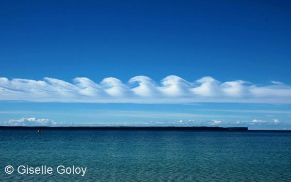
4. If $\rho_{-0} \gtrsim \rho_{+0}$, $k_{crit} \approx 0$, and KH is very common in these systems. There are many applications of this case, but on important one is fast moving dry air over slower moving, water-laden air over the ocean. This gives rise to billow clouds.

In Astrophysics:

AGN jets, or stellar jets, moving at high speed relative to the surrounding medium often display KH instabilities.

Thermal Instabilities

First, heat conduction – the transportation of heat (i.e., thermal energy) from hot to cold regions. In the simplest case, there is no mass motion, unlike convection. An empirical relation has been found, but it’s hard to derive from first principles. This relation is called Fourier’s Law of Heat Conduction.

$$\boxed{\underbrace{\vec F}_\text{heat flux} = -\underbrace{k}_\text{thermal conductivity} \underbrace{\vec \nabla T}_\text{temperature gradient}}$$

Note that heat flux has units of $\text{energy}/(\text{Area} \cdot \text{ time})$, and thus thermal conductivity has units of $\text{Watts}/(\text{m}\cdot \text{ Kelvin})$. Here are some example values:

• Air : $k = 0.024 \text{ W } \text{ m}^{-1} \text{K}^{-1}$

• Aluminum has $k=200$

• Copper has $k=400$

• Diamond has $k=1000$ or so…

• Nano tubes/graphene sheets are a bit more special.

For our fluid equations, we will:

1. Turn on Thermal Conduction & Cooling/Heating. 2. Ignore gravity.

Our fluid equations become:

$$\frac{\partial \rho}{\partial t} + \vec \nabla \cdot (\rho \vec v) = 0$$

$$\frac{\partial \vec v}{\partial t} + (\vec v \cdot \vec \nabla) \vec v = -\frac{1}{\rho} \vec \nabla P$$

$$\frac{\partial \varepsilon}{\partial t} + \vec \nabla \cdot \vec F = \dot{Q}$$

where $\dot{Q}$ represents other heating rates (per volume) and $\varepsilon$ is the thermal energy density. The third equation can be re-written:

$$\frac{\partial \varepsilon}{\partial t} = \vec \nabla (k \vec \nabla T) + \dot{Q}$$

We can perturb the three equations above, which we won’t do here (see Pringle & King Ch. 8, or Clarke & Carswell Ch. 9, or Field (1965, ApJ)).

Skipping the math, we can quote the result:

For thermal instability to occur, we need:

$$\left(\frac{\partial \dot{Q}}{\partial T}\right)\Bigg\vert_\text{const. P} > 0 \rightarrow \text{ The Field Criterion}$$

This makes sense since, as $T$ increases slightly, net $\dot{Q}$ increases, meaning that we heat the material even more! This is the instability.

An Example

Consider the interstellar medium (ISM). We will write heating/cooling rates as:

$$\dot{Q} = \underbrace{\dot{Q}_{+}}_\text{heating} - \underbrace{\dot{Q}_{-}}_\text{cooling}$$

The typical cooling curve looks something like this:

NEED IMAGE FROM NOTES HERE

We thus have three phases of the ISM. When the ISM is near $T_{1}$ (cool phase) in some regions. $T_{3}$ (hot phase) is stable in other regions. This gives rise to multiphase ISM!

Comments

1. There is an E&M analogy to Fourier’s Law – this is Ohm’s Law!:

$$\vec J = \sigma \vec E$$

since the electric field can be written as the gradient of the electric potential.

2. Thermal Energy Conservation:

$$\frac{\partial \varepsilon}{\partial t} + \vec \nabla \cdot \vec F = 0$$

where $\varepsilon$ is the energy density. and $\vec F$ is the heat flux we introduced above. Note that $\varepsilon \propto T$ most of the time, and thus we have:

$$\frac{\partial T}{\partial t} \propto \nabla^2 T$$

which is a diffusion equation. We diffuse heat transfer due to $e^{-}$-nuclei collisions.

3. This is hard to derive from first principles since this is a non-equilibrium process. But, people work on that!

previous

Waves