Energy Transport in Stars¶

Radiation Transport¶

Consider a hot material (say, inside a star), with some boundary, and more gas on the other side of the boundary. The gas interior emits photons, some of which crossing the boundary. The gas outside the boundary is slightly cooler, and still emitting photons.

How do we describe the photons and where they go? Because we have a temperature gradient, the photons are flowing from interior to exterior the boundary. We can think of this movement as a diffusion – in reality, it is not the same photon random walking, but we will treat it as such.

Radiative Transfer Refresher¶

We care about two basic properties of the photons and the material:

Intensity of the radiation
Matter opacity (absorbativity/transparency).

We can define our specific intensity \(I(\theta)\mathrm{d}\theta\), where \(\theta\) is the direction of radiation and \(\mathrm{d}\Omega\) is the solid angle over which the photon is emitted:

\[ I(\theta) = \frac{\text{erg}}{\text{s cm}^2 \text{ str Hz}} \]

We want to relate our flux to our specific intensity:

\[ F = \int I \cos\theta \mathrm{d}\Omega = \int_0^{2\pi} \int_{0}^{\pi} I(\theta, \phi)\cos\theta \cdot \sin\theta \mathrm{d}\theta\mathrm{d}\phi \]

Absorption¶

What we really care about is the actually observed flux, and we must account for the opacity \(\kappa\):

\[ \kappa = \frac{\text{cm}^2}{g} \]

You can think of this as a per-mass cross section.

We can write our equation of radiative transfer thus us:

\[ \mathrm{d}I = -I \kappa \rho \mathrm{d}s \]

The initial intensity is modulated by the opacity and the thickness.

We can solve:

\[ \boxed{I = I_0 e^{-\kappa \rho s}} \]

We will commonly see something called \(\tau \equiv \kappa \rho s\), which is the optical depth.

Emission¶

What happens if our slab is actually emitting more than it absorbs? We have some slab emission rate \(j_\nu\). Note that:

\[ [j_\nu] = \frac{\text{ergs}}{\text{s cm}^3 \text{ sr Hz}} \]

This modifies our radiation equation and we instead have:

\[ \frac{\mathrm{d}I}{\mathrm{d}s} = - I \kappa \rho + j \]

Often, we see:

\[ \boxed{\frac{dI}{d\tau} = - I + S \text{ where } j_\nu \equiv \frac{j}{\kappa \rho}} \]

A Treatment of Stars¶

We are now talking about slabs at a radius \(r\) from the center of the star in the direction \(\hat z\). The slab thickness is thus \(dz\). We have:

\[ \frac{dI(z,\theta)}{ds} = \frac{\cos\theta \cdot \mathrm{d}I(z,\theta)}{\mathrm{d}z} \]

Note we are implicitly assuming that the density is constant here, which in exotic cases, is not true.

So….how the hell do we progress? Let’s

Assume a blackbody at tempertature \(T \rightarrow\) we can say that the source function is uniform in all directions (locally). Note that the lower the mass, and the cooler the star, the more this assumption breaks down. This gives us, where \(S(T)\) is the Planck Fucntion, that:

\[ I(z,\theta) = S(T) - \frac{\cos\theta}{\kappa \rho}\frac{\mathrm{d}I(z,\theta)}{\mathrm{d}z} \]

Note that we can solve this equation by assuming that \(I(z,\theta) = B(T) + \underbrace{\epsilon I(z,\theta)}_\text{small perturbation}\). Fundamentally, after treating this as a perturbation, we end up with:

\[ H_\nu = \int I(z,\theta)\cos\theta \mathrm{d}\Omega = \int \left(B(T) - \frac{\cos\theta}{\kappa \rho} \frac{dB(T)}{dz}\cos\theta \right)\mathrm{d}\Omega \]

\[ H_\nu = \int \left(\underbrace{B(T)}_\text{integral goes to 0} - \frac{\cos\theta}{\kappa \rho} \frac{dB(T)}{dz}\cos\theta \right)\mathrm{d}\Omega \]

\[ H_\nu = -\frac{2\pi}{\kappa \rho} \frac{dB(T)}{dz}\int_0^\pi \cos^2\theta \sin\theta \mathrm{d}\theta \]

This becomes:

\[ H_\nu = -\frac{4\pi}{3\kappa \rho} \frac{dB(T)}{dz} = -\frac{4\pi}{3\kappa\rho}\frac{\partial B}{\partial T}\frac{\partial T}{\partial z} \]

And the total flux is thus:

\[ H = -\frac{4\pi}{3\rho} \frac{\partial T}{\partial z} \int_0^\infty \frac{1}{\kappa}\frac{\partial B(T)}{\partial T}\mathrm{d}\nu \]

Note that the integral is nasty. The opacity is a WILD FUNCTION of quantum mechanics, resonances, etc. Almost always, things like MESA hide the complexity of microphysics in the integral.

We want to hide this nastiness, and how do we make this tractable? Let’s define a quantity called the Rosseland Mean Opacity \(\kappa_R\) such that:

\[ \frac{1}{\kappa_R} \equiv \frac{\int_0^\infty \frac{1}{\kappa}\frac{\partial B(T)}{\partial T}\mathrm{d}\nu}{\int_0^{\infty} \frac{\partial B(T)}{\partial T} \mathrm{d}\nu} = \frac{\pi}{4\sigma T^3}\int_0^\infty \frac{1}{\kappa}\frac{\partial B(T)}{\partial T}\mathrm{d}\nu \]

This can be thought of as a mean transparency, or so, and often ignore the complex treatments underneath. This is normally fine for stuctures, but not for specific spectra in atmospheres. When we do this, we can go back to the total flux per unit area of a shell from a star:

\[ \boxed{H = -\frac{16\sigma T^3}{3\kappa_R \rho}\frac{\partial T}{\partial z}} \]

What we actually observe is integrated over the full sphere:

\[ \boxed{L(r) = -4\pi r^2 \frac{16 \sigma T^3}{3\kappa_R \rho}\frac{dT}{dz}} \]

A Note on the Lagrangian Formalism¶

What if we want the temperature gradient in terms of mass instead of radius? We have:

\[ \boxed{\frac{dT}{dr} = \frac{-3}{16\sigma}\frac{\kappa \rho}{T^3}\frac{L(r)}{4\pi r^2}} \]

We can also do this for mass:

\[ \boxed{\frac{dT}{dm} = \frac{-3}{16\sigma} \frac{\kappa_R}{T^3} \frac{L(r)}{\left(4\pi r^2\right)^2}} \]

We can also think of this as (approximately):

\[ \frac{dT}{dm} \propto L_{below} \kappa_R \]

Combining Our Temperature and Pressure Gradients with HE¶

Our temperature gradient is:

\[ \frac{dT}{dm} = \underbrace{\frac{dP}{dm}}_{\text{from HE, }=\frac{GM}{4\pi r^2}}\frac{dT}{dP} \]

Substitute in:

\[ \frac{dT}{dm} = -\frac{Gm}{4\pi r^4} \frac{T}{P}\frac{\mathrm{d}\ln T}{\mathrm{d}\ln P} \]

We will define a dimensionless quantity:

\[ \nabla_\text{rad}\equiv \left(\frac{\partial \ln T}{\partial \ln P}\right)_\text{rad} \]

\[ \nabla_\text{rad} = -\frac{P}{T}\frac{4\pi r^2}{Gm}\frac{3\kappa_R}{4ac \left(4\pi\right)^2}\frac{1}{T^3}\frac{L(r)}{r^4} \]

We can simplify, giving:

\[ \boxed{\nabla_\text{rad} = \frac{3\kappa_R}{16\pi ac G}\frac{LP}{mT^4}} \]

Conceptually, this is log variation of T with depth. Note that this still has an idela gas equation of state, but radiative diffusion is the dominant energy transport. This is subtle! Note that \(\kappa_R\) and convection vs. diffusion are the dominant differences in strucutre between high and low mass stars.

A Note on Rosseland Mean Opacity¶

What are some various \(\kappa_R\)’s?

Electron Scattering¶

The general picture is that we have an ionized medium at low \(\rho\) and low \(T\). We have to have electrons and thus have some ionization. A photon comes in and scatters off the electron, giving an opacity. Thomson scattering is non-relativistic (and an elastic scatter process). Compton is relaivistic.

This happens in the outer envelopes of stars, with \(T > 10,000\) K. We also need to have photons which are not relativistic – thus \(h\nu < 0.1 m_e c^2\) or so, and so \(T<10^{8}\) K or so. Note that this temperature range is basically the entire star, **so if we have to do first order calculations, we assume Thomson opacity and modify from there. **

\[ \sigma_T = 6.6\times 10^{-25} \text{cm}^2 \]

with \(\kappa = \sigma_t/\mu m_p\).

This gives

\[ \kappa_R = \frac{\sigma_T}{\mu m_{unit mass}} = 0.2\left(1+X\right) \text{ g }^{2} \text{ cm }^{-1} \]

Free-Free Absorption¶

I covered this. Make sure to go get the notes.

Bound-Free (Ionization)¶

Here, we have an atom with an electron bound. A photon comes in and makes it free. We thus need:

\[ E_{photon} > E_{binding} \]

Note that this is typically not hydrogen, but this is affecting the metals.

\[ \kappa_{BF} = 4.35\times 10^{25} g_{bf} Z(1+X)(\rho/\text{ g }\text{ cm}^3)(T/K)^{-7/2} cm^2/g \]

Another thing to consider:

\[ \kappa_{bf} \sim 10^{3} Z \kappa_{ff} \]

Bound free and free free happen, sort of, in the same regime because metals are typically 1% or so. We can’t have \(T>10^{4}\) K or so, because we don’t want to be fully ionized. We also want a meatl reach environment, with something like \(Z>10^{-3}\) or so.

H- Opacity¶

Note that in astronomy, we have a very weird ion. If we have an area of a lot of free electrons, and a really high density so that we can force the protons to hang out with the electrons.

This is extremely fragile. Even though it is fragile – when it does exist, it has an opacity:

\[ \kappa_{H-} \sim 10^{-31} \left(\frac{Z}{0.02}\right)\rho^{1/2} T^{9} \frac{\text{cm}^2}{\text{g}} \]

The opacity can SKYROCKET with high temperatures. This is most relevant for the outer parts of low mass stars. When the temperature is \(T\gtrsim 3000-6000 \) K, and when \(T<10,000\) K (so we are not ionized), and when we have metals \(Z\sim > 10^{-2.5}\). In this regime, H- is a dominant form of opacity! Because this is the outermost layer, this is the regulating layer. Thus, what we are actually seeing is set byt he opacity at the outer layer.

Other Opacity: Molecules and Dust¶

Relevant for really, really cool stars and in their outermost layers
Relevant for star formation, not as much for main sequence and post-main sequence though.

Convection¶

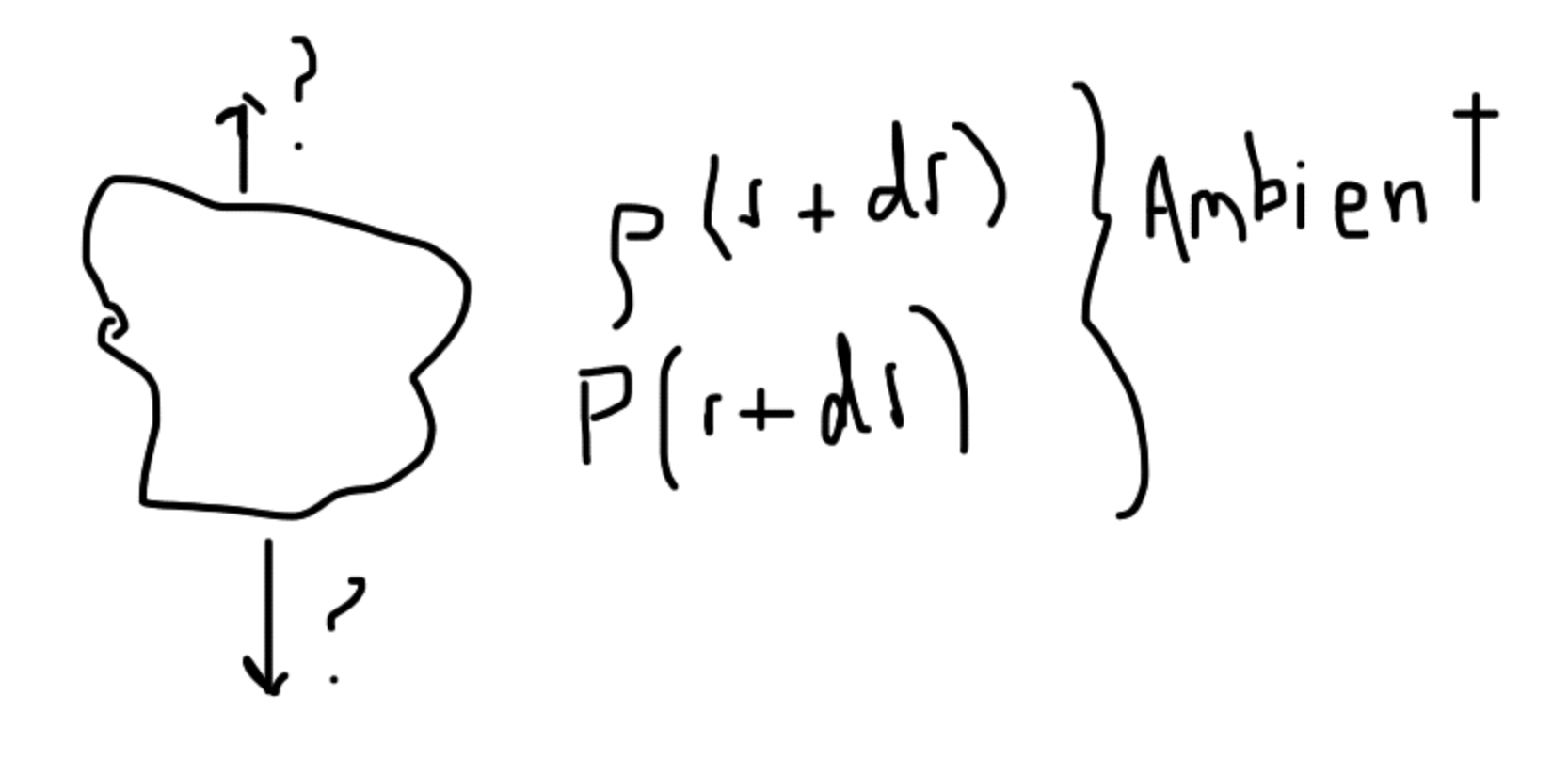
Consider a blob of gas with some radius \(r\), some pressure \(P(r)\), and some density \(\rho(r)\). We will displace our blob of gas upward a bit, and see what happens. This radius is now \(r+\mathrm{d}r\), and the ambient conditions of this blob are different – \(P\rightarrow P(r+\mathrm{d}r)\) and \(\rho\rightarrow \rho(r+\mathrm{d}r)\). This is almost impossible to solve, unless we use the adiabatic assumption: assume that the gas responds in an adibatic way. This means we have no heat transfer in the star. We are assuming this locally, by the way, which is why this might seem counter intuitive. In other words, we are expanding this blob adiabatically – only changing the size of the blob.

In this end, this will lead to an expression for \(dP/dr\) and \(dT/dr\) under these conditions, giving an equivalent \(\nabla_{ad}\). We then compare the two gradients, and whichever is more efficient will win!

The Basic Questions¶

We don’t really understand convection. We need to know where convection happens.

Our problem last time: we have a blob of gas with some properties. This blob moves somewhere else (different ambient conditions), how does it respond?

In the case when \(\rho_{internal} < \rho(r+dr)\), we get a new upward force. This is an instability.
When \(\rho_{internal} > \rho_{ambient}\), then we have a net downward force.

All we need to do is figure out the internal density. Starting with the ideal gas law:

\[ P = \frac{\rho}{\mu} T \mathcal{R} \text{ where } \mathcal{R} \equiv 3.8\times 10^{7} \frac{\text{g}\text{cm}^2}{\text{s}^2 \text{ K} \text{ mole}} \equiv \frac{\text{erg}}{\text{K} \text{ Mole}} \]

Let’s take a derivative, assuming a constant \(\mu\):

\[ \frac{dP}{dr} = \frac{\mathcal{R}}{\mu} \left(\rho \frac{dT}{dr} + T\frac{d\rho}{dr}\right) \]

Plugging back in for \(\rho\) in terms of pressure and temperature.

\[ \frac{dP}{dr} = = \left(\frac{P}{T}\frac{dT}{dr} + \frac{P}{\rho}\frac{d\rho}{dr}\right) \]

We now have to assume that the gas is adiabatic. Then, by definition, we have: \(P = \mathcal{K} \rho^\gamma\). We can now plug this in to hopefully get rid of the density dependence above.

Taking the derivative:

\[ \frac{dP}{dr} = \mathcal{K}\gamma \rho^{\gamma-1} \frac{d\rho}{dr} \rightarrow \frac{dP}{dr} = \gamma \frac{P}{\rho} \frac{d\rho}{dr} \]

Combine our two equations (ideal gas + adiabatic gas conditions), then solve for the tempearture gradient:

Setting the two pressure gradients equal:

\[ \gamma \frac{P}{\rho} \frac{d\rho}{dr} = \left(\frac{P}{T}\frac{dT}{dr} + \frac{P}{\rho}\frac{d\rho}{dr}\right) \]

Simplifying:

\[ \frac{dT}{dr} = \left(\gamma-1\right)\frac{P}{\rho}\left(\frac{d\rho}{dr}\right)\frac{T}{P} = (\gamma-1)\frac{T}{\rho}\frac{d\rho}{dr} \]

Swapping for pressure:

\[ \frac{dT}{dr}= \boxed{\underbrace{\frac{\gamma-1}{\gamma}\frac{T}{P}\frac{dP}{dr} \equiv \left(\frac{dT}{dr}\right)_{ad}}_\text{adiabatic temperature gradient}} \]

The next steps are very messy, but we basically write \(F=ma\) with densities. Fundamentally, we idenify that:

Condition for the Instability and Hence Convection¶

This condition is met when:

\[ \boxed{\frac{dT}{dr} < \left(\frac{dT}{dr}\right)_{ad} \rightarrow \text{Convection.}} \]

Conceptually, this is confusing because of the signs. We can re-write these conditions to be more intuitive:

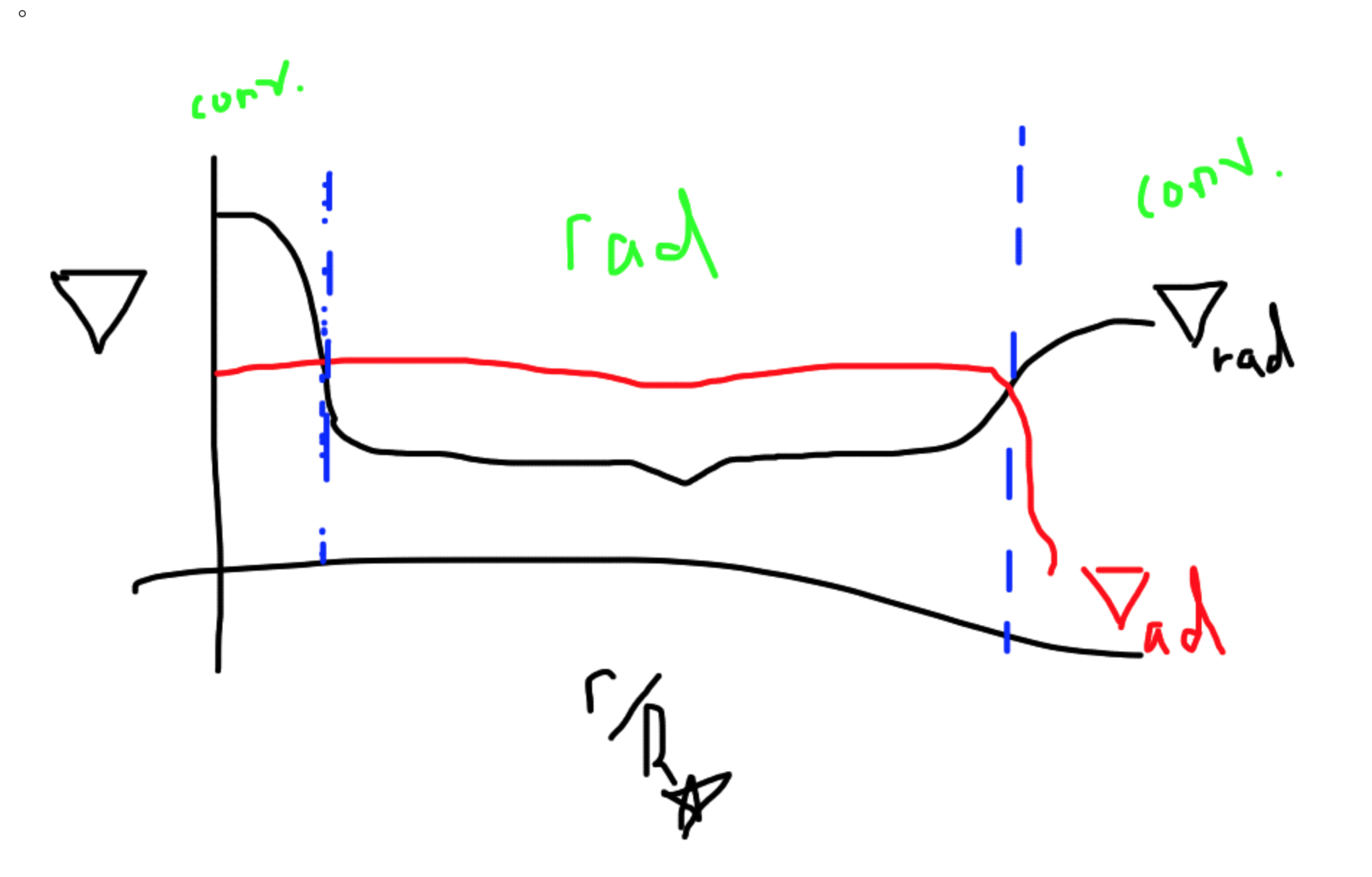
\[ \boxed{\Bigg| \frac{dT}{dr}\Bigg| > \Bigg|\frac{dT}{dr}\Bigg|_{ad}} \]

This basically says that if the true temperature gradient is STEEPER than the adiabatic condition, we get convection.

Remember earlier we had:

\[ \nabla \equiv \frac{d\ln T}{d\ln P} \]

When we had this expression, we flip signs and require for convection (same idea as above but with a sign flip).

\[ \boxed{\nabla > \nabla_{ad}} \]

Some notes:¶

The condition:

\[ \boxed{\frac{\gamma-1}{\gamma} < \frac{3 \kappa_R L(r) P }{16 \pi ac G m T^4} \rightarrow \text{ Convection}} \]

If \(\kappa_R\) increases, we have more convection.
When \(L/M\) (energy generation efficiency) increases, we are also more convective.

Homologous Stars¶

Here’s an exercise useful for scaling relations. We will treat all differentials as differences. We want scaling relations between parameters. We will treat \(\rho \sim \frac{M}{R^3}\).

Hydrostatic Equilibrium

\[ P \sim \frac{GM^2}{R^4} \]

Ideal Gas Law

\[ T \sim \frac{\mu GM}{R} \]

Energy Transport (Radiative Star)

\[ L \sim \frac{R^2}{\kappa \rho}\frac{T^4}{R} \]

Opacity

\[ \kappa \sim \rho^{n} T^{-\alpha} \]

which is true for many forms of the opacity.

Starting with the luminosity:

\[ L \sim R^2 \underbrace{\frac{R^3}{M}}_{\rho} \underbrace{\left(\frac{R^3}{M}\right)^n \left(\frac{\mu G M}{R}\right)^{\alpha}}_{\kappa} \underbrace{\left(\frac{\mu GM}{R}\right)^{4}}_{T^4} \frac{1}{R} \]

We are left with things that we can measure! Collecting our terms:

\[ \boxed{L \sim \mu^{\alpha+4} R^{3n-\alpha} M^{\alpha+3-n}} \]

This is great for quick, order-of-magnitude calculations.

Examples¶

Kramer’s Opacity (Free-Free Opacity) + Ideal Gas¶

Here, we have: \(\alpha=7/2\) and \(n=1\). In this case, we have:

\[ \boxed{L \sim \mu^{7.5} R^{-1/2} M^{5.5}} \]

If the whole star is dominated by Kramer’s opacity,

Thomson Opacity¶

In this case, the opacity is constant and we have:

\[ L \sim \mu^{4} M^3 \]

Thomson opacity is appropriate for the most massive stars.

Radiation Pressure and Thomson Opacity¶

Here, we have:

\[ P \sim P_R \sim \frac{GM^2}{R^4} \]

And thus:

\[ L \sim R^2 \frac{R^3}{M} \frac{GM^2}{R^5} \sim M \]

These are the most massive stars where radiation pressure matters. We have linear relation between mass and luminosity.

Stellar Astrophysics

Energy Transport in Stars

Contents