.ipynb .pdf

repository open issue

Binder

Contents

Fitting a Line to Data

import numpy as np
import matplotlib.pyplot as plt
import matplotlib as mpl
mpl.rcParams['font.size'] = 16
mpl.rcParams['legend.fontsize'] = 14
mpl.rcParams['figure.dpi'] = 150

Linear Least Squares with Matrices

Let’s fit a line of the form:

$$y = \beta_0 x + \beta_1$$

Assuming that both y and x are vectors with $n$ elements, we can rewrite this equation in matrix form:

$$\begin{split} \begin{bmatrix} Y_1 \\ Y_2 \\ \vdots \\ Y_n \end{bmatrix} = \begin{bmatrix} \beta_0 + \beta_1 X_1 \\ \beta_0 + \beta_1 X_2 \\ \vdots \\ \beta_0 + \beta_1 X_n \end{bmatrix} \end{split}$$

$$\begin{split} \underbrace{\begin{bmatrix} Y_1 \\ Y_2 \\ \vdots \\ Y_n \end{bmatrix}}_{Y_{n\times1}} = \underbrace{\begin{bmatrix} 1 & X_1 \\ 1 & X_2 \\ \vdots & \vdots \\ 1 & X_n \end{bmatrix}}_{X_{n\times2}} \underbrace{\begin{bmatrix} \beta_0 \\ \beta_1 \end{bmatrix}}_{\beta_{2\times1}} \end{split}$$

$$Y = X \beta$$

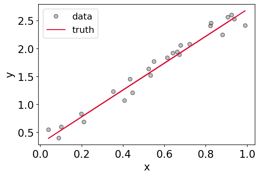
Here, I’ll simulate some data with $n=25$:

# generate some random, linear data with random error
n = 25
x = np.random.uniform(size=n)
y = 2.4*x + 0.3 + np.random.normal(0,0.1,size=n)

# plot the data
plt.figure()
plt.plot(x,y,'o',label = 'data',mfc='gray',markeredgecolor='k',alpha=0.5)
plt.plot(x,2.4*x + 0.3,label = 'truth',color='crimson')
plt.xlabel('x')
plt.ylabel('y')
plt.legend()

<matplotlib.legend.Legend at 0x7fe37733f490>

We can now directly solve for the vector $\beta$ after reshaping our data to the matrix shapes above:

$$\hat{\beta}=\left(X^{T} X\right)^{-1} X^{T} Y$$

# first reshape to make these the proper matrix forms
Y = y.reshape((-1,1)) # 100 x 1
# add a vector of ones as a column to X (see above equation)
vector_of_ones = np.ones(n)
X = np.column_stack((vector_of_ones, x))

print('X shape: ', X.shape)
print('Y shape: ', Y.shape)

X shape:  (25, 2)
Y shape:  (25, 1)

beta_hat = np.linalg.inv(X.T @ X) @ X.T @ Y
print('Beta Shape: ', beta_hat.shape)

Beta Shape:  (2, 1)

beta_hat

array([[0.32544314],
       [2.38931179]])

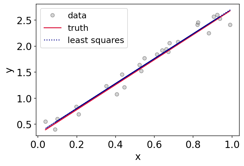
# generate a best fit line
x_fit = np.linspace(0,1,10)
y_fit = beta_hat[1]*x + beta_hat[0]

# plot the data, best fit line, and ground truth
plt.figure()
plt.plot(x,y,'o',label = 'data',mfc='gray',markeredgecolor='k',alpha=0.33)
plt.plot(x,2.4*x + 0.3,label = 'truth',c='crimson')
plt.plot(x,y_fit,label='least squares',c='darkblue',ls='dotted')
plt.xlabel('x')
plt.ylabel('y')
plt.legend()

<matplotlib.legend.Legend at 0x7fe377a4c810>

Weighted Least Squares

What if our data have measurement errors which are not constant? How do we weight our points properly?

We can slightly modify our expression for $\beta$ above in the case of known measurement errors. For more math, see Section 2.2 of: https://www.stat.cmu.edu/~cshalizi/mreg/15/lectures/24/lecture-24–25.pdf.

Another great resource: https://adrian.pw/blog/fitting-a-line/

The result is that we can define a weight matrix $W = diag(1/\sigma_i)$ where $\sigma_i$ are the measurement errors for the $i$th measurement. In this case, we have:

$${\displaystyle {\hat {\boldsymbol {\beta }}}=(X^{\textsf {T}}WX)^{-1}X^{\textsf {T}}W\mathbf {y} .}$$

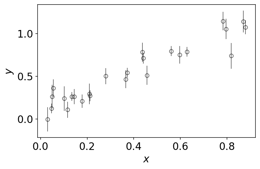
# generate some random, linear data with random error
n = 25
x = np.random.uniform(size=n)

# evaluate the true model at the given x values
y = 1.17*x + 0.1

# Heteroscedastic Gaussian uncertainties only in y direction
y_err = np.random.uniform(0.05, 0.15, size=n) # randomly generate uncertainty for each datum
y = np.random.normal(y, y_err) # re-sample y data with noise

datastyle = dict(mec='k', linestyle='none',ecolor='k', marker='o', mfc='none', label='data',alpha=0.6,elinewidth=1)
plt.figure()
plt.errorbar(x, y, y_err, **datastyle)
plt.xlabel('$x$')
plt.ylabel('$y$')
plt.tight_layout()

# solve for beta after defining our matrices
# data matrix
Y = y.reshape((-1,1)) # 50 x 1

# design matrix
vector_of_ones = np.ones(n)
X = np.column_stack((vector_of_ones, x))

# weight matrix
W = np.diag(1/y_err**2)

# solve for beta
beta_hat_weighted = np.linalg.inv(X.T @ W @ X) @ X.T @ W @ Y
beta_hat_unweighted = np.linalg.inv(X.T @ X) @ X.T @ Y

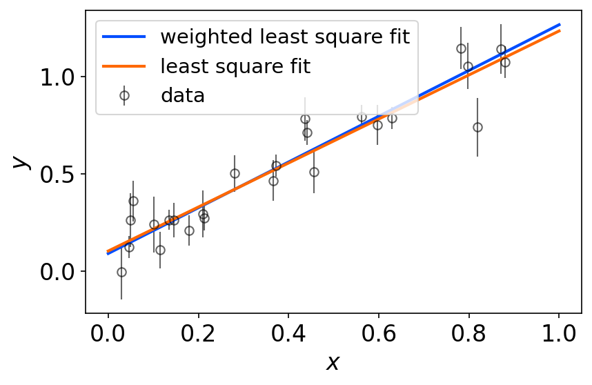
print(f'Weighted Least Squares:\t  y = {np.round(float(beta_hat_weighted[1]),4)}x+{np.round(float(beta_hat_weighted[0]),4)}')
print(f'Unweighted Least Squares: y = {np.round(float(beta_hat_unweighted[1]),4)}x+{np.round(float(beta_hat_unweighted[0]),4)}')

Weighted Least Squares:	  y = 1.175x+0.0903
Unweighted Least Squares: y = 1.1302x+0.103

# generate a best fit line
x_fit = np.linspace(0,1,10)
y_fit_weighted = beta_hat_weighted[1]*x_fit + beta_hat_weighted[0]
y_fit_unweighted = beta_hat_unweighted[1]*x_fit + beta_hat_unweighted[0]

cmap = plt.get_cmap('jet')
dictstlye = dict(mec='k', linestyle='none',ecolor='k', marker='o', mfc='none', label='data',alpha=0.6,elinewidth=1)
plt.figure()
plt.errorbar(x, y, y_err, **dictstlye)
plt.plot(x_fit,y_fit_weighted,color=cmap(0.2/1),label='weighted least square fit',lw=2)
plt.plot(x_fit,y_fit_unweighted,color=cmap(0.8/1),label='least square fit',lw=2)
plt.xlabel('$x$')
plt.ylabel('$y$')
plt.legend(loc='upper left')
plt.tight_layout()

previous

Matrix Operations with Numpy

next

Maximum Likelihood